
243
CHAPTER 18
TEACHING NOTES
Several of the topics in this chapter, including testing for unit roots and cointegration, are now
staples of applied time series analysis. Instructors who like their course to be more time series
oriented might cover this chapter after Chapter 12, if time permits. Or, the chapter can be used
as a reference for ambitious students who wish to be versed in recent time series developments.
Example 18.5 tests for cointegration between the general fertility rate and the value of the
personal exemption. There is not much evidence of cointegration, which sheds further doubt on
the regressions in levels that were used in Chapter 10. The error correction model for holding
yields in Example 18.7 is likely to be of interest to students in finance. As a class project, or a
term project for a student, it would be interesting to update the data to see if the error correction
model is stable over time.
244
SOLUTIONS TO PROBLEMS
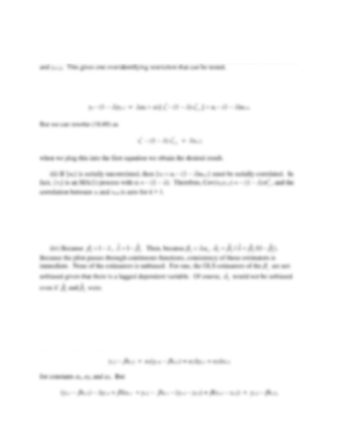
18.1 With zt1 and zt2 now in the model, we should use one lag each as instrumental variables, zt-1,1
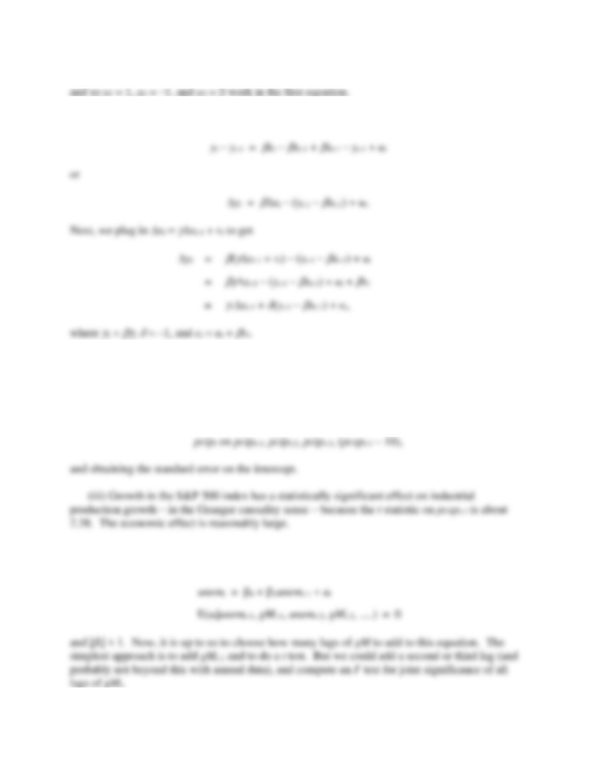
18.2 (i) When we lag equation (18.68) once, multiply it by (1 –
), and subtract it from (18.68),
we obtain
(iii) Because {vt} follows an MA(1) process, it is correlated with the lagged dependent
variable, yt-1. Therefore, the OLS estimators of the
j will be inconsistent (and biased, of course).
Nevertheless, we can use xt-2 as an IV for yt-1 because xt–2 is uncorrelated with vt (because ut and
ut-1 are both uncorrelated with xt-2) and xt-2) and xt-2 is partially correlated with yt-1.
18.3 For
, yt –
zt = yt –
zt + (
–
)zt, which is an I(0) sequence (yt –
zt) plus an I(1)
sequence. Since an I(1) sequence has a growing variance, it dominates the I(0) part, and the
resulting sum is an I(1) sequence.
18.4 Following the hint, we show that yt-2 –
xt-2 can be written as a linear function of yt-1 –
xt-1,
yt-1, and xt-1. That is,
245
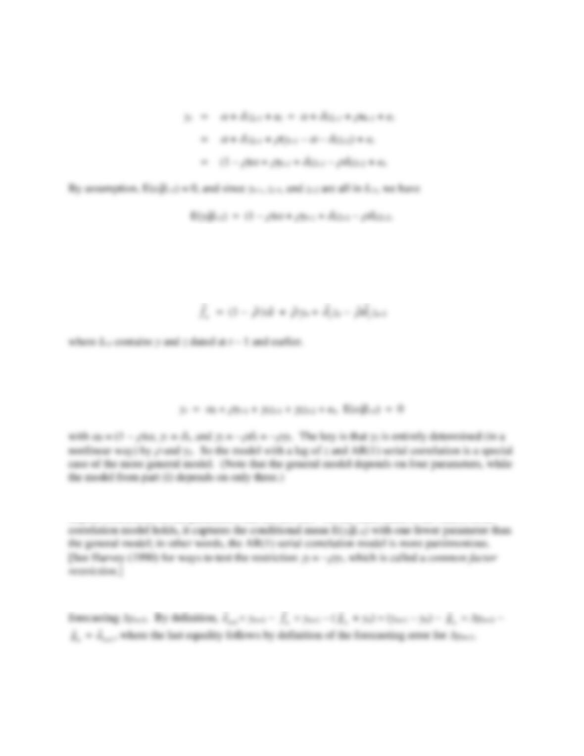
18.5 Following the hint, we have
18.6 (i) This is given by the estimated intercept, 1.54. Remember, this is the percentage growth
at an annualized rate. It is statistically different from zero since t = 1.54/.56 = 2.75.
(ii) 1.54 + .031(10) = 1.85. As an aside, you could obtain the standard error of this estimate
by running the regression.
pcipt on pcipt-1, pcipt-2, pcipt-3, (pcspt-1 – 10),
18.7 If unemt follows a stable AR(1) process, then this is the null model used to test for Granger
causality: under the null that gMt does not Granger cause unemt, we can write
246
18.8 (i) Following the hint we have
We obtain the desired answer by adding one to the time index everywhere.
(ii) The forecasting equation for yn+1 is obtained by using part (i) with t = n, and then
plugging in the estimates:
(iii) From part (i), it follows that the model with one lag of z and AR(1) serial correlation in
the errors can be obtained from
(iv) For forecasting, the AR(1) serial correlation model may be too restrictive. It may
impose restrictions on the parameters that are not met. On the other hand, if the AR(1) serial
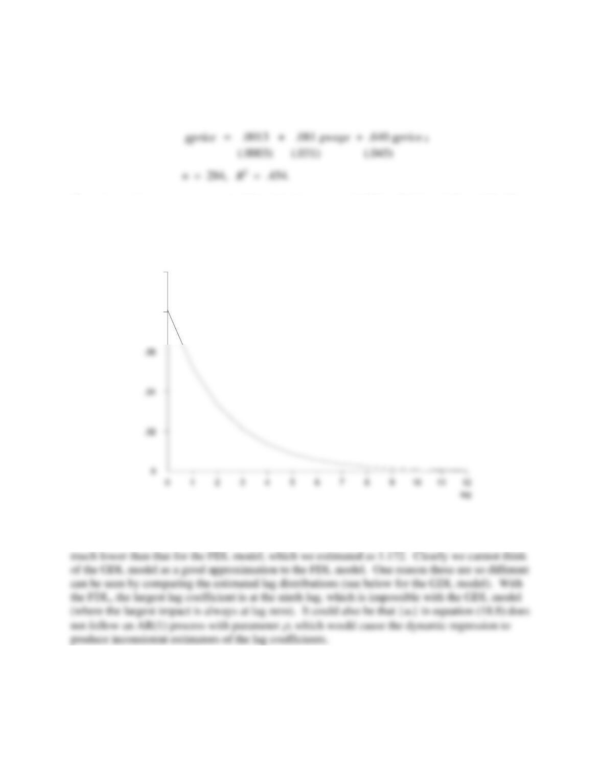
18.9 Let
1
ˆn
e+
be the forecast error for forecasting yn+1, and let
1
ˆn
a+
be the forecast error for
247
SOLUTIONS TO COMPUTER EXERCISES
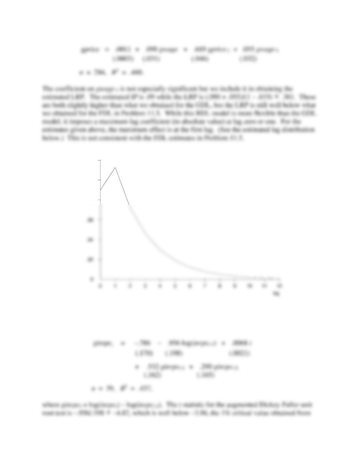
C18.1 (i) The estimated GDL model is
The estimated impact propensity is .081 while the estimated LRP is .081/(1 – .640) = .225. The
estimated lag distribution is graphed below.
(ii) The IP for the FDL model estimated in Problem 11.5 was .119, which is substantially
above the estimated IP for the GDL model. Further, the estimated LRP from GDL model is
(iii) When we estimate the RDL from equation (18.16) we obtain
.08
coefficient .1
248
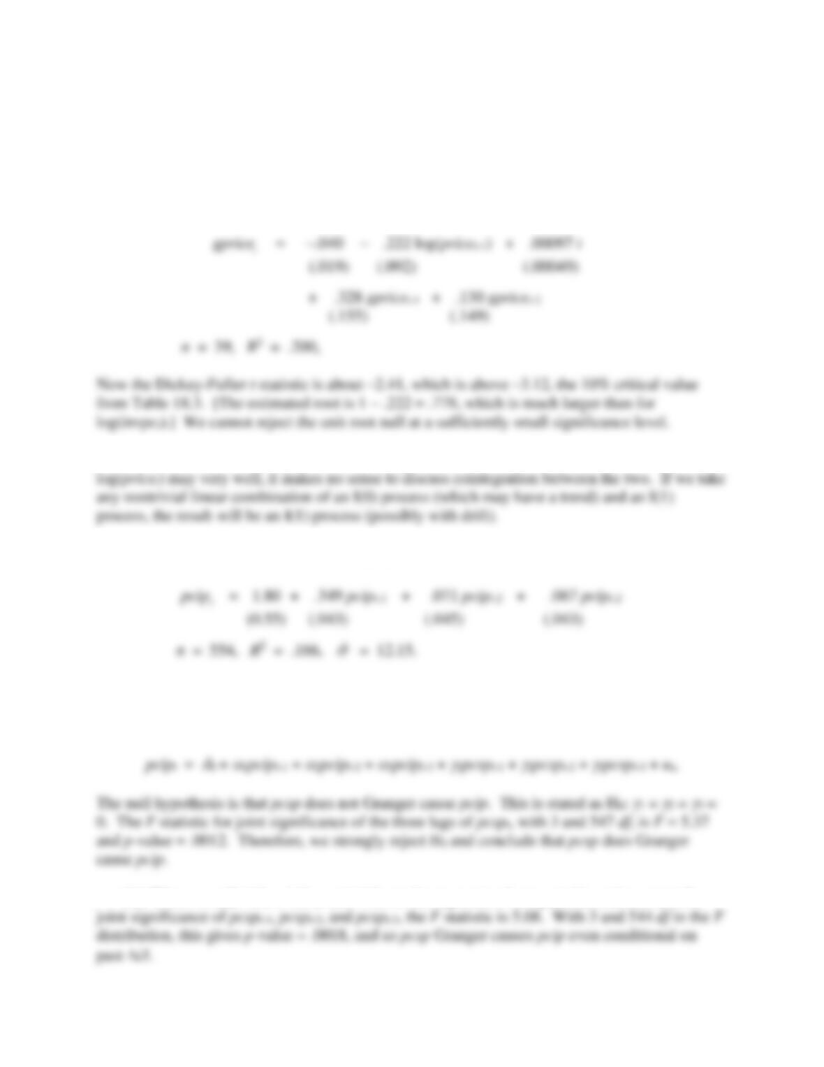
C18.2 (i) We run the regression
.08
.1
coefficient .12
249
Table 18.3. Therefore, we strongly reject a unit root in log(invpct). (Incidentally, remember that
the t statistics on the intercept and time trend in this estimated equation to not have approximate t
distributions, although those on ginvpct-1 and ginvpct-2 do under the usual null hypothesis that the
parameter is zero.)
(ii) When we apply the regression to log(pricet) we obtain
(iii) Given the very strong evidence that log(invpct) does not contain a unit root, while
C18.3 (i) The estimated AR(3) model for pcipt is
When pcipt-4 is added, its coefficient is .0043 with a t statistic of about .10.
(ii) In the model
pcipt =
(iii) When we add i3t-1, i3t-2, and i3t–3 to the regression from part (ii), and now test the
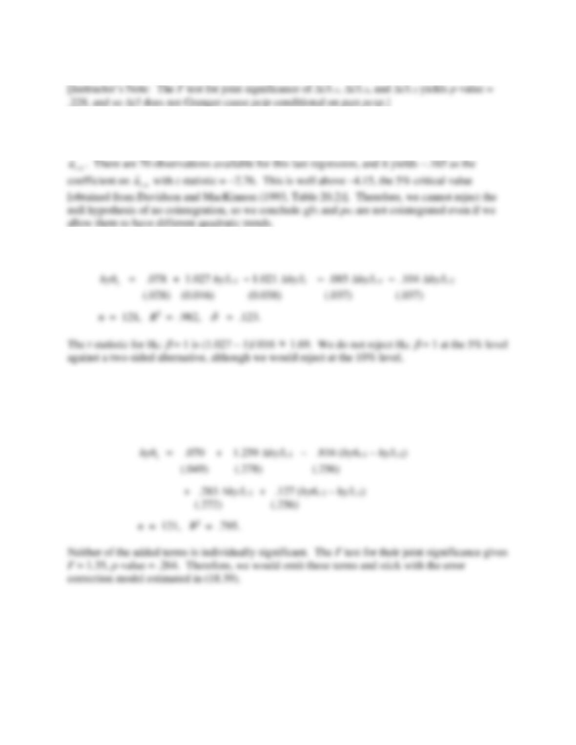
250
C18.4 We first run the regression gfrt on pet, t, and t2, and obtain the residuals,
ˆt
u
. We then
apply the augmented Dickey-Fuller test, with one lag of
ˆt
u
, by regressing
ˆt
u
on
1
ˆt
u−
and
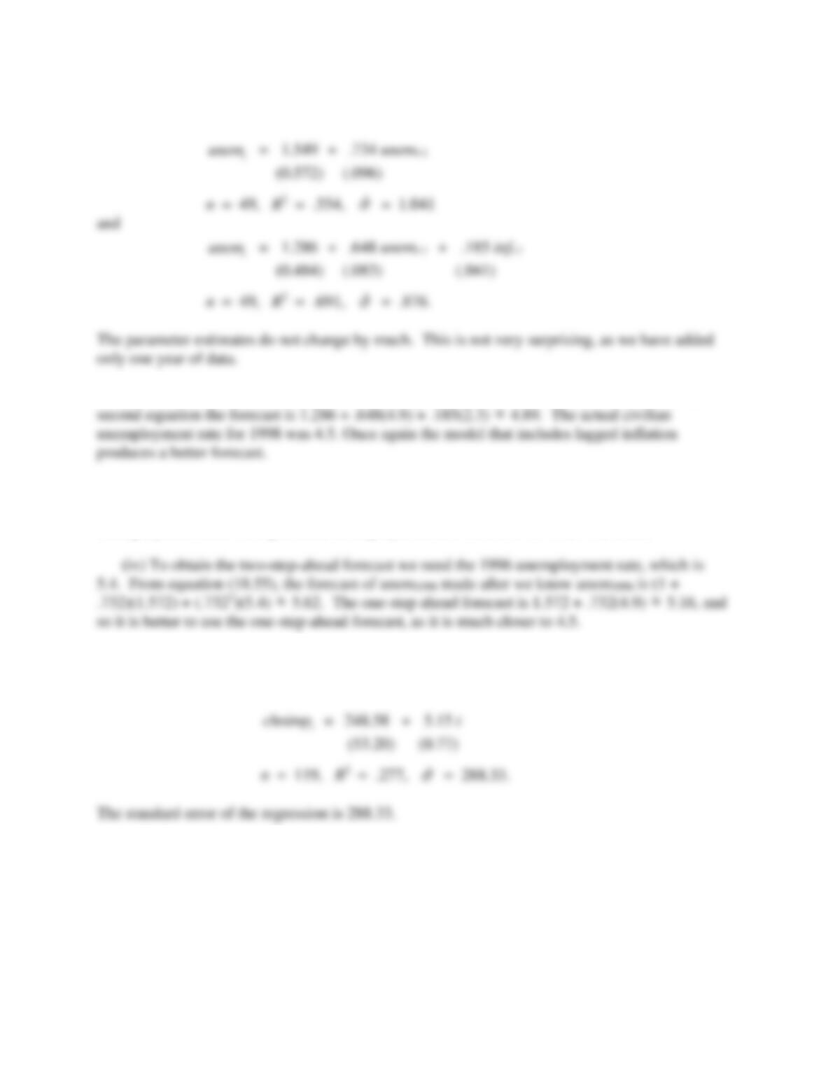
C18.5 (i) The estimated equation is
[Instructor’s Note: The standard errors on all slope coefficients can be used to construct t
statistics with approximate t distributions, provided there is no serial correlation in {et}.]
(ii) The estimated error correction model is
251
C18.6 (i) The equations using data through 1997 are
(ii) The forecast for unem1998 from the first equation is 1.549 + .734(4.9)
5.15; from the
(iii) There is no practical improvement in reestimating the parameters using data through
1997: 4.89 versus 4.90, which differs in a digit that is not even reported in the published
unemployment series: our predicted unemployment rate would be 4.9% in both cases.
C18.7 (i) The estimated linear trend equation using the first 119 observations and excluding the
last 12 months is
(ii) The estimated AR(1) model excluding the last 12 months is
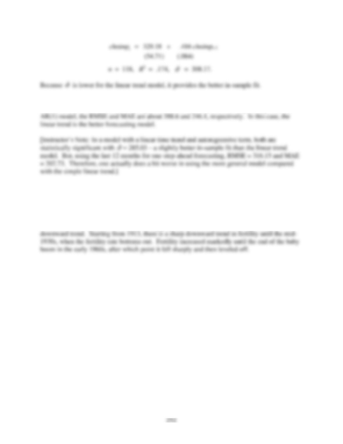
(iii) Using the last 12 observations for one-step-ahead out-of-sample forecasting gives an
RMSE and MAE for the linear trend equation of about 315.5 and 201.9, respectively. For the
(iv) Using again the first 119 observations, the F statistic for joint significance of febt, mart,
…, dect when added to the linear trend model is about 1.15 with p-value
.328. (The df are 11
and 107.) So there is no evidence that seasonality needs to be accounted for in forecasting
chnimp.
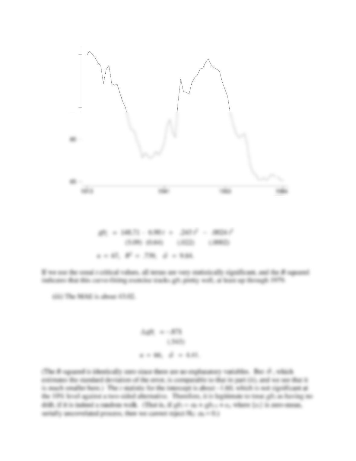
C18.8 (i) As can be seen from the following graph, gfr does not have a clear upward or
253
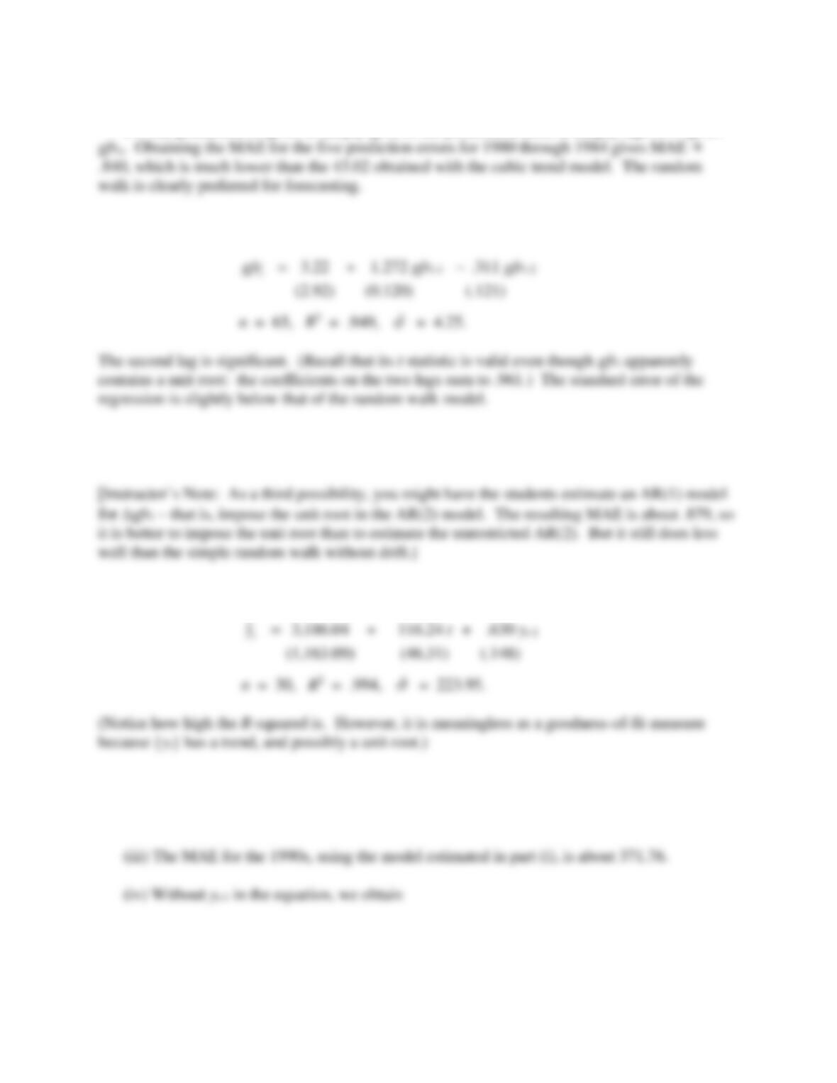
(ii) The regression of gfrt on a cubic in t, using the data up through 1979, gives
(iv) The regression gfrt on just an intercept, using data up through 1979, gives
year
100
gfr 125
254
(v) The prediction of gfrn+1 is simply gfrn, so the predication error is simply gfrn+1 = gfrn+1 –
(vi) The estimated AR(2) model for gfrt is
(vii) The out-of-sample forecasting performance of the AR(2) model is worse than the
random walk without drift: the MAE for 1980 through 1984 is about .991 for the AR(2) model.
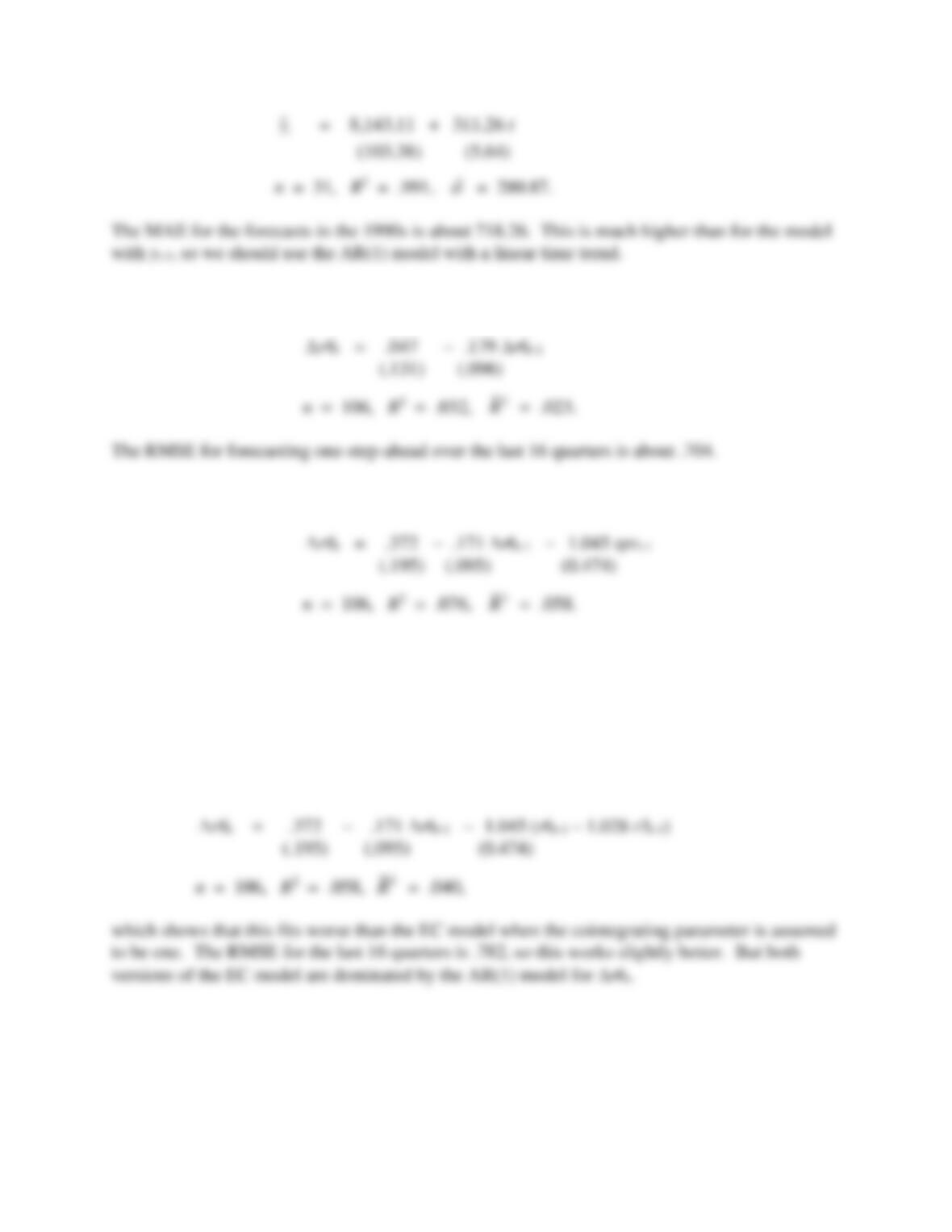
C18.9 (i) Using the data up through 1989 gives
(ii) The forecast for 1990 (t = 32) is 3,186.04 + 116.24(32) + .630(17,804.09)
18,122.30,
because y is $17,804.09 in 1989. The actual value for real per capita disposable income was
$17,944.64, and so the forecast error is –$177.66.
255
C18.10 (i) The AR(1) model for r6, estimated using all but the last 16 observations, is
(ii) The equation with sprt-1 included is
The RMSE is about .788, which is higher than the RMSE without the error correction term.
Therefore, while the EC term improves the in-sample fit (and is statistically significant), it
actually hampers out-of-sample forecasting.
(iii) To make the forecasting exercises comparable, we exclude the last 16 observations to
estimate the cointegrating parameters. The CI coefficient is about 1.028. The estimated error
correction model is
[Instructor’s Note: Because r6t-1 is only marginally significant in the AR(1) model, its
coefficient is small, and the intercept is also very small and insignificant, you might have the
students use zero to predict r6 for each of the last 16 quarters. In other words, the “model” for
r6 is simply
6tt
ru=
, where
t
u
is an unpredictable sequence with zero mean. The resulting
256
(iv) The conclusions would be identical because, as shown in Problem 18.9, the one-step-
ahead errors for forecasting r6n+1 are identical to those for forecasting r6n+1.
C18.11 (i) For lsp500, the ADF statistic without a trend is t = −.79; with a trend, the t statistic is
−2.20. This are both well above their respective 10% critical values. In addition, the estimated
roots are quite close to one. For lip, the ADF statistic without a trend is −1.37 without a trend
and −2.52 with a trend. Again, these are not close to rejecting even at the 10% levels, and the
estimated roots are very close to one.
(ii) The simple regression of lsp500 on lip gives
(iii) Using the residuals
ˆt
u
obtained in part (ii), the ADF statistic (with two lagged changes)
(iv) After adding a linear time trend to the regression from part (ii), the ADF statistic applied
(v) It appears that lsp500 and lip do not move together in the sense of cointegration, even if
C18.12 (i) The F statistic for the second and third lags, with 2 and 550 degrees of freedom, gives
F = 3.76 and p-value = .024.
257
C18.13 (i) The DF statistic is about −3.31, which is to the left of the 2.5% critical value (−3.12),
and so, using this test, we can reject a unit root at the 2.5% level. (The estimated root is about
.81.)
(iv) The best characterization seems to be an I(0) process about a linear trend. In fact, a
stable AR(3) about a linear trend is suggested by the regression in part (iii).
an I(0) process whether or not we include a trend.
C18.14 (i) Using the ADF regression with one lag and a time trend, the coefficient on
1
232t
lwage −
is only −.0056 with t = −1.39. The estimated root is so close to one (.9944) that the
(ii) Without a time trend, the regression
112
ˆ ˆ ˆ ˆ
on , ,
t t t t
u u u u
− − −
(where the
ˆt
u
are the
(iii) If we use the real wage, as defined in the problem, and include a time trend, the
coefficient on
1
ˆt
u−
is −.044 with t = −3.09. Now, at least the estimated root is less than one
258
C18.15 (i) The usual DF test, obtained by regressing curate on a lag of urate, gives a very
small coefficient, −.0063, and a t statistic, −.79, that is not close to being significant. Adding two
lags of curate changes little: The coefficient on urate_1 becomes −.0086 with t = −1.22. There is
very little evidence against the unit root hypothesis for urate. The coefficients on both lags of
curate are positive and statistically very significant, but the outcome of the augmented DF test is
essentially the same as the usual DF test.
(ii) For vrate the outcome is less clear cut. From the simple DF regression, the estimated 𝜌 is
about .925. The DF t = −2.68, is below the 10% critical value, −2.57, but above the 5% critical
(iii) To implement the Engle-Granger test for cointegration, we regress urate on vrate and get
(iv) We obtain the leads-and-lags estimator of
by regressing
urate
on
vrate
,
cvrate
,
(v) When two lags are added to the EG regression, the t statistic falls dramatically in
magnitude: t = −1.05. Now there is no evidence of cointegration, which is particularly troubling