Economics Chapter 18 Homework The Monthly Payment 540 The Real Value

Unlock access to all the studying documents.

View Full Document

CHAPTER 18

Inflation, the Phillips Curve, and

Central Bank Commitment

KEY IDEAS IN THIS CHAPTER

2. The Freidman-Lucas money surprise model predicts a positive relationship between

3. The model also predicts that the Phillips curve is unstable, as it shifts with the

changes in the expected inflation rate.

5. The central bank learning hypothesis provides a more plausible explanation than the

central bank commitment hypothesis, as it seems difficult to argue that the Bank of

NEW IN THE FOURTH EDITION

1. All data and graphs have been updated.

TEACHING GOALS

Phillips curves play a prominent role in New Keynesian analysis, so it is useful to know

whether they are observed in the data or not. One way to generate a Phillips curve, not

unlike the mechanism at work in sticky price models, is in a Friedman-Lucas money

surprise model, studied in this chapter. The most important points in this chapter are that

a) stable Phillips curves, if they exist at all, are only short-run phenomena, and that b)

policymakers’ attempts to exploit the Phillips curve may lead to a permanent increase in

inflation and at best a temporary increase in aggregate output.

The primary subject of this chapter is to develop a positive theory of inflation. In the

short run, central banks face a given level of expected inflation. Over time, policy

behaviour affects the future course of expectation formation. The interplay of central

Chapter 18: Inflation, the Phillips Curve, and Central Bank Commitment

bank behaviour and the behaviour of the public generates the equilibrium rate of

CLASSROOM DISCUSSION TOPICS

Public discussion periodically focuses on whether the Bank of Canada should be given

less discretion. This topic was given more attention during the 1970s and early 1980s

when the Bank of Canada allowed the rate of inflation become higher than what the

public was willing to tolerate. On the one hand, if the Bank of Canada is charged only

with controlling the rate of inflation and given clear performance standards, theory

suggests the rate of inflation will remain closer to its preferred level. On the other hand,

discretion may be needed for the Bank of Canada to respond properly to macroeconomic

disturbances. How do students feel about giving the Bank of Canada less discretion? How

does the answer to this question depend on students’ judgments about the validity of

competing theories of the business cycle?

There is some conflict between the Friedman-Lucas money surprise model of the Phillips

curve and the assumed properties of central bank preferences. In particular, the model

assumes that the central bank always prefers higher output. However, if the Friedman-

Lucas model is correct, then aggregate output can be above trend only when workers are

fooled into working more hours than they would actually prefer. Can increases in output

due to erroneous decisions be welfare improving? Is it possible that a more Keynesian-

style model of the Phillips curve is a better justification for these preferences? Are there

other factors that might cause the socially optimal level of aggregate output to be higher

than the level of output consistent with equality between actual inflation and expected

inflation? What might these factors be?

Most countries’ tax systems are not perfectly indexed for inflation. They impose taxes on

nominal, not real, returns on investments (bonds and stocks), which distorts the prices on

those assets. Also, capital gains are taxed in nominal terms, so investors may pay a big

tax on assets whose value has not increased in real terms.

To see this in a simple example (with the simplifying assumption that the real return, not

the after-tax real return, is fixed), consider two cases in which there is a 30% tax rate.

Instructor’s Manual for Macroeconomics, Fourth Canadian Edition

seems consistent with the data.) A solution to this problem is to adjust capital values for

inflation before taxing them.

Mortgage loans are most often made at fixed rates for long terms. When inflation is

positive, the constant nominal payment over time is much higher in real terms early in the

life of the loan and lower in real terms later in the life of the loan, because of a higher

A numerical example illustrates this. Consider a $100,000, 30-year mortgage. In case A

the inflation rate is 0% and the nominal interest rate is 5%. The monthly payment is $540,

the real value of which is constant over time. Using the 28% rule used by lenders (that a

person’s mortgage payment shouldn’t exceed 28% of income), a person requires an

OUTLINE

1. The Phillips Curve

a) The Work of A.W. Phillips

b) The Phillips Curve in Canada

i) A Stable Phillips Curve: 1962–1979 and 1990–2005

c) The Behaviour of Phillips Curves across Time and Space

i) Phillips Curves do not Exist in all Data Sets

ii) Phillips Curves Appear to Shift over Time

2. Money Surprises and the Phillips Curve

3. A Positive Theory of Inflation

a) Central Bank Preferences

b) Central Bank Maximization for Given Expectations

Chapter 18: Inflation, the Phillips Curve, and Central Bank Commitment

c) Long-Run Equilibrium

d) The Role of Commitment

i) Time Inconsistency

4. Central Bank Learning

5. Central Bank Commitment

a) The Bank of Canada

b) Commitment to Low Inflation in Hong Kong (Macroeconomics in Action 17.2)

TEXTBOOK QUESTION SOLUTIONS

Problems

1. Initially, the inflation rate is equal to i* and aggregate output is equal to YT. The

initial Phillips curve is PC1. To exploit PC1 optimally, the central bank adopts the

inflation rate i1, and the level of aggregate output increases to Y1. In the next

Figure 17.1

2. Disinflation.

a) The economy starts at the point (YT, i1) in Figure 17.2a. The expected rate of

inflation is i1, and the relevant Phillips curve is PC1. To reduce inflation to i*

Figure 17.2a

Chapter 18: Inflation, the Phillips Curve, and Central Bank Commitment

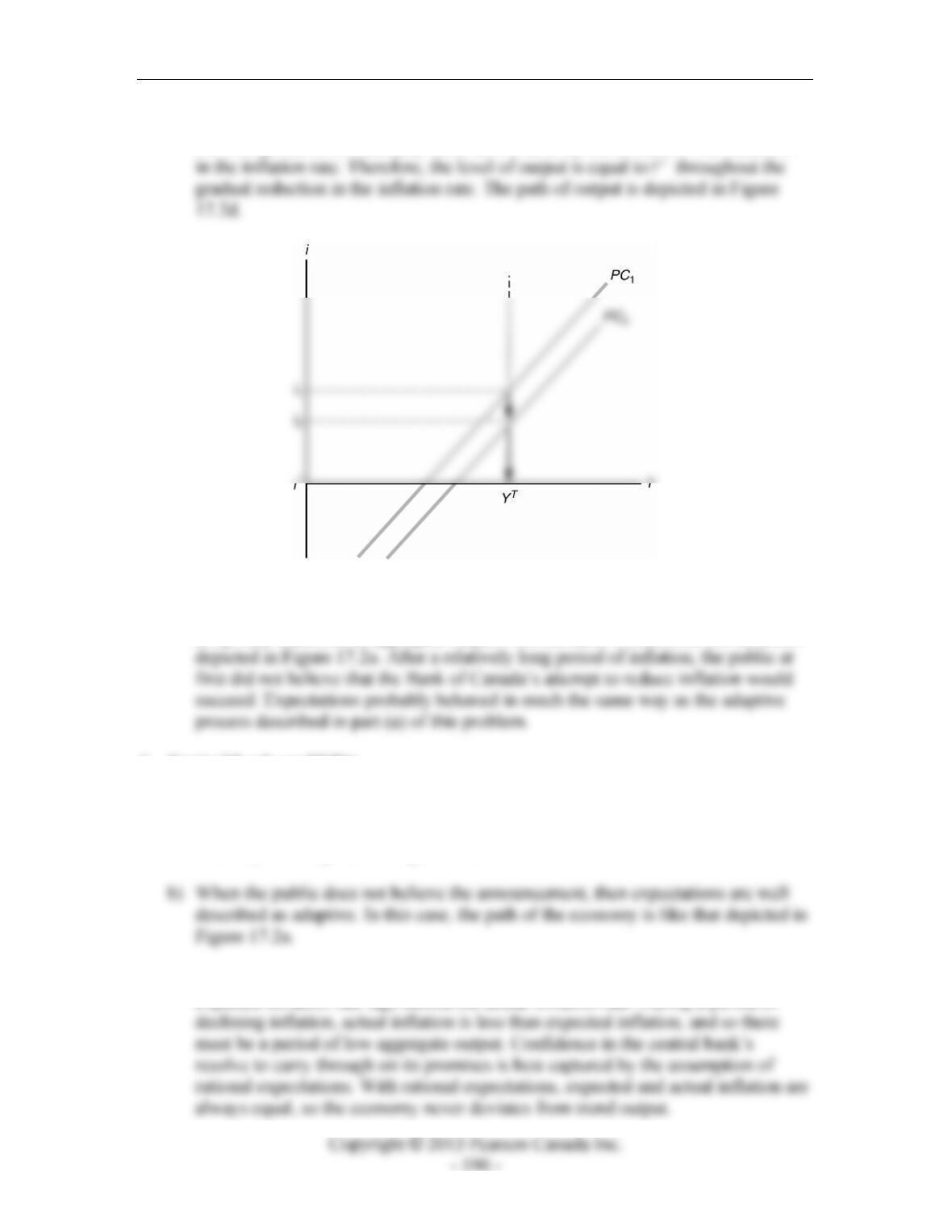
b) With rational expectations, the expected rate of inflation immediately declines to

i*. The economy immediately moves to the point (YT, i*) in Figure 17.2b.

Therefore, the economy does not have to endure a period of low output to end the

excessive inflation.

Figure 17.2b

c) The economy starts at the point (YT, i1) in Figure 17.2c. If the central bank first

reduces the inflation rate to 2

i, and expectations are adaptive, output declines to 2

Figure 17.2c

Instructor’s Manual for Macroeconomics, Fourth Canadian Edition

If expectations are rational, then with each gradual step down in the inflation rate,

the Phillips curve immediately shifts downwards by the amount of the reduction

Figure 17.2d

d) In the early 1980s, the inflation rate fell dramatically, and there was a large,

temporary reduction in aggregate output. This scenario is much like the transition

3. Central bank credibility.

a) When the public has confidence that the central bank will follow through on its

promise, then expectations are well described as rational. Movement in the

economy is as depicted in Figure 17.2b.

c) When expectations are slow to adapt, there is a period of time during which the

expected inflation rate lags behind the actual inflation rate. During a period of