Chapter 18
Discrete Choices and Event Counts
◼ Exercises
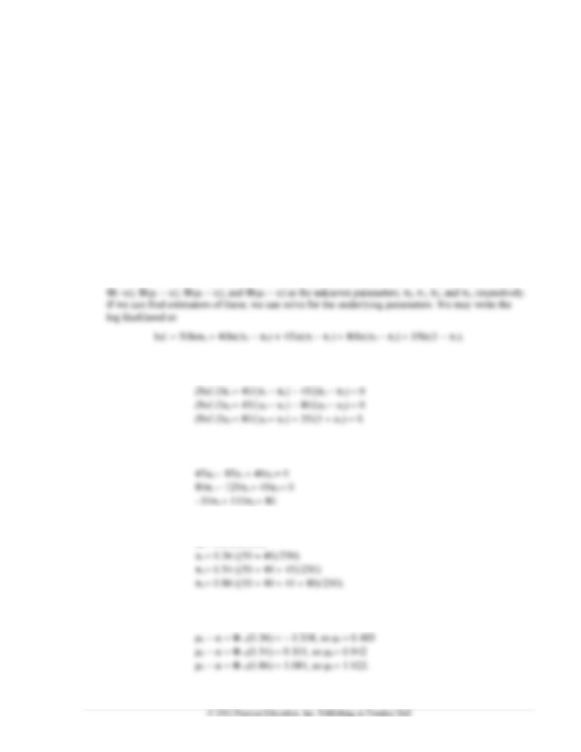
1. Since there is no regressor, we may write the log likelihood as
lnL = 50ln(−) + 40ln[(μ1 − ) − (−)] + 45ln[(μ2 − ) − (μ1 − )] +
80ln[(μ3 − ) − (μ2 − )] + 35ln[1 − (μ3 − )].
There are four unknown parameters to estimate and four free probabilities. Suppose, then, we treat
The necessary conditions are
lnL/0 = 50/0 − 40/(1 − 0) = 0
By a simple rearrangement, these can be recast as a set of linear equations. Thus,
900 − 501 = 0
The solution (as might be expected) is
0 = 0.2 (50/250)
Now, we can solve for the underlying parameters.
− = −1(0.2) = − 0.841, so = 0.841
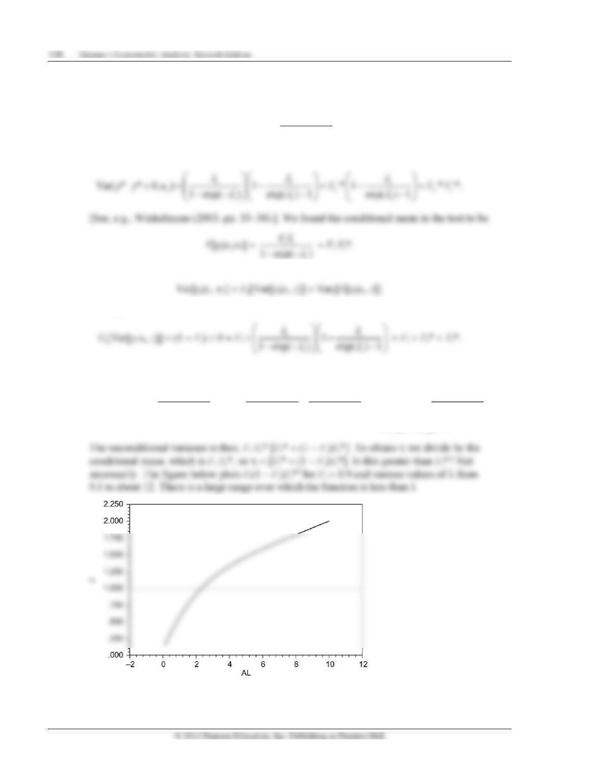
2. (a) Conditional variance in the ZIP model. The essential ingredients that are needed for this
derivation are
*
[ *| * 0, ] 1 exp( )
i
ii
i
E y y E
= =
−−
x
and
i
To obtain the variance, we will use the variance decomposition,
The expectation of the conditional variance is
The variance of the conditional mean is
(1 − Fi)
−
−−
2
01 exp( )
ii
i
F
+ Fi
−
− − − −
2
1 exp( ) 1 exp( )
i i i
ii
F
= Fi(1 − Fi)
−−
2
1 exp( )
i
i
= Fi(1 − Fi)Ei*2.
Chapter 18 Discrete Choices and Event Counts 139
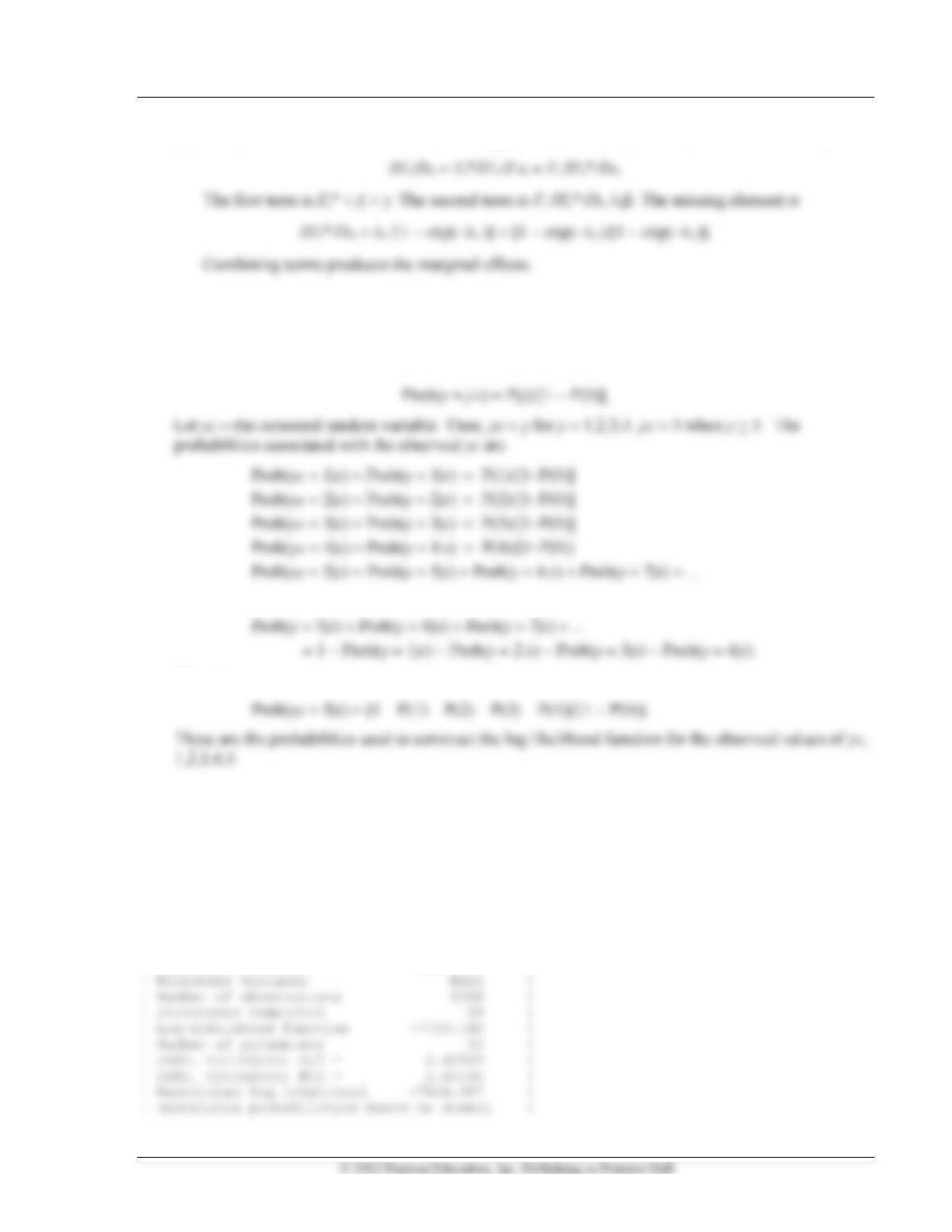
(b) Partial Effects. The mean is Fi Ei*. We suppose that wi and xi are the same for the moment,
3. Let y* denote the unobserved random variable that is distributed as Poisson with probability
Prob(y* = j|x) = P( j) = exp(−)j/j!.
The observed random variable before the censoring is y = y*|y*> 0. The probabilities are
The last term is an infinite sum. But,
Therefore,
Applications
Application 18.1 is the same as Application 17.1.
?========================================================================
? Application 18.2 Ordered Choice for Self-Reported Marriage Rating
?========================================================================
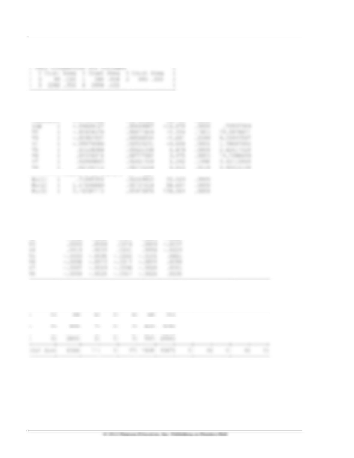
+———————————————+
| Ordered Probability Model |
| Maximum Likelihood Estimates |
| Dependent variable MARRIAGE |
140 Greene • Econometric Analysis, Seventh Edition
+———————————————+
+———————————————+
| Ordered Probability Model |
+———————————————+
+——–+————–+—————-+——–+——–+———-+
|Variable| Coefficient | Standard Error |b/St.Er.|P[|Z|>z]| Mean of X|
+——–+————–+—————-+——–+——–+———-+
———+Index function for probability
Constant| 1.87997564 .12760529 14.733 .0000
———+Threshold parameters for index
+————————————————————————-+
| Summary of Marginal Effects for Ordered Probability Model (probit) |
+————————————————————————-+
Variable| Y=00 Y=01 Y=02 Y=03 Y=04 Y=05 Y=06 Y=07 |
————————————————————————–+
YRB .0031 .0087 .0167 .0093 -.0377
V2 .0002 .0006 .0011 .0006 -.0024
+—————————————————————————+
| Cross tabulation of predictions. Row is actual, column is predicted. |
| Model = Probit . Prediction is number of the most probable cell. |
+——-+——-+—–+—–+—–+—–+—–+—–+—–+—–+—–+—–+
| Actual|Row Sum| 0 | 1 | 2 | 3 | 4 | 5 | 6 | 7 | 8 | 9 |
+——-+——-+—–+—–+—–+—–+—–+—–+—–+—–+—–+—–+
| 1| 348| 2| 0| 5| 170| 171|
| 3| 2242| 3| 0| 10| 674| 1555|
Chapter 18 Discrete Choices and Event Counts 141
?===================================================
? Application 18.3
?===================================================
Namelist ;x = age,educ,hhninc,hsat $
Poisson ; Lhs = HospVis ; Rhs = One,X
; Marginal effects $
Calc ; Lp = logl $
—————————————————-
Sample ; All $
Regress ; Lhs = one ; Rhs = one ; Str = ID ; Panel $
Poisson ; Lhs = HospVis ; Rhs = One,X
; Marginal effects
+———————————————+
| Poisson Regression |
| Maximum Likelihood Estimates |
| Dependent variable HOSPVIS |
| Weighting variable None |
+———————————————+
| Poisson Regression |
+———————————————+
+——–+————–+—————-+——–+——–+———-+
|Variable| Coefficient | Standard Error |b/St.Er.|P[|Z|>z]| Mean of X|
+——–+————–+—————-+——–+——–+———-+
Constant| .12613692 .12567036 1.004 .3155
142 Greene • Econometric Analysis, Seventh Edition
+——–+————–+—————-+——–+——–+———-+
|Variable| Coefficient | Standard Error |b/St.Er.|P[|Z|>z]| Mean of X|
+——–+————–+—————-+——–+——–+———-+
Constant| .01743926 .02183573 .799 .4245
AGE | -.00047111 .00025979 -1.813 .0698 43.5256898
HSAT | -.03442771 .00220148 -15.638 .0000 6.78542607
+—————————————————-+
| Ordinary least squares regression |
| LHS=HOSPVIS Mean = .1382566 |
| Standard deviation = .8843390 |
+—————————————————-+
+——–+————–+—————-+——–+——–+———-+
|Variable| Coefficient | Standard Error |b/St.Er.|P[|Z|>z]| Mean of X|
+——–+————–+—————-+——–+——–+———-+
Constant| .49839670 .04097910 12.162 .0000
AGE | -.00064393 .00048945 -1.316 .1883 43.5256898
+———————————————+
| Negative Binomial Regression |
| Dependent variable HOSPVIS |
+———————————————+
+——–+————–+—————-+——–+——–+———-+
|Variable| Coefficient | Standard Error |b/St.Er.|P[|Z|>z]| Mean of X|
+——–+————–+—————-+——–+——–+———-+
Constant| .10394982 .12631220 .823 .4105
AGE | -.00369348 .00143149 -2.580 .0099 43.5256898
+——————————————-+
| Partial derivatives of expected val. with |
| respect to the vector of characteristics. |
| Effects are averaged over individuals. |
+——————————————-+
Chapter 18 Discrete Choices and Event Counts 143
+——–+————–+—————-+——–+——–+———-+
|Variable| Coefficient | Standard Error |b/St.Er.|P[|Z|>z]| Mean of X|
+——–+————–+—————-+——–+——–+———-+
Constant| .01421398 .02120646 .670 .5027
?===================================================
? Application 18.4
?===================================================
+———————————————+
| Panel Model with Group Effects |
| Dependent variable HOSPVIS |
| Weighting variable None |
| Number of observations 27326 |
+———————————————+
+——–+————–+—————-+——–+——–+———-+
|Variable| Coefficient | Standard Error |b/St.Er.|P[|Z|>z]| Mean of X|
+——–+————–+—————-+——–+——–+———-+
AGE | -.00020613 .00705126 -.029 .9767 43.5256898
+——————————————-+
| Partial derivatives of expected val. with |
| respect to the vector of characteristics. |
| They are computed at the means of the Xs. |
+——————————————-+
+——–+————–+—————-+——–+——–+———-+
|Variable| Coefficient | Standard Error |b/St.Er.|P[|Z|>z]| Mean of X|
+——–+————–+—————-+——–+——–+———-+
AGE | -.284995D-04 .00097488 -.029 .9767 1.00000000
+———————————————+
| Panel Model with Group Effects |
| Dependent variable HOSPVIS |
144 Greene • Econometric Analysis, Seventh Edition
+———————————————+
+——–+————–+—————-+——–+——–+———-+
|Variable| Coefficient | Standard Error |b/St.Er.|P[|Z|>z]| Mean of X|
+——–+————–+—————-+——–+——–+———-+
Constant| -.22178663 .13617622 -1.629 .1034
AGE | -.00170639 .00145901 -1.170 .2422 43.5256898
+——————————————-+
| Partial derivatives of expected val. with |
| respect to the vector of characteristics. |
+——————————————-+
+——–+————–+—————-+——–+——–+———-+
|Variable| Coefficient | Standard Error |b/St.Er.|P[|Z|>z]| Mean of X|
+——–+————–+—————-+——–+——–+———-+
Constant| -.03066347 .01882726 -1.629 .1034
?===================================================
? Application 18.5 Ship Accidents
?===================================================
+———————————————+
| Poisson Regression |
| Dependent variable ACC |
| Number of observations 34 |
+———————————————+
+———————————————+
| Poisson Regression |
| Chi-squared = 39.70580 RsqP= .9491 |
+———————————————+
+——–+————–+—————-+——–+——–+———-+
|Variable| Coefficient | Standard Error |b/St.Er.|P[|Z|>z]| Mean of X|
+——–+————–+—————-+——–+——–+———-+
LOGMTH | .90617018 .10174566 8.906 .0000 7.04925451
Chapter 18 Discrete Choices and Event Counts 145
T7074 | .39874282 .20053445 1.988 .0468 .29411765
O6074 | -.36986273 .11821010 -3.129 .0018 .41176471
+———————————————+
| Poisson Regression |
| Maximum Likelihood Estimates |
| Dependent variable ACC |
| Number of observations 34 |
+———————————————+
| Poisson Regression |
+———————————————+
+——–+————–+—————-+——–+——–+———-+
|Variable| Coefficient | Standard Error |b/St.Er.|P[|Z|>z]| Mean of X|
+——–+————–+—————-+——–+——–+———-+
LOGMTH | 1.00000000 ……(Fixed Parameter)…….
Constant| -5.25351861 .24642858 -21.319 .0000
There is no evidence of overdispersion. The tests from the Poisson model are both
insignificant, and the estimate of in the negative binomial model is essentially zero.
+———————————————+
| Negative Binomial Regression |
| Dependent variable ACC |
| Weighting variable None |
+———————————————+
+——–+————–+—————-+——–+——–+———-+
|Variable| Coefficient | Standard Error |b/St.Er.|P[|Z|>z]| Mean of X|
+——–+————–+—————-+——–+——–+———-+
LOGMTH | 1.00000000 ……(Fixed Parameter)…….
Constant| -5.25074235 .26830333 -19.570 .0000
TA | -.32296435 .39695609 -.814 .4159 .20588235

146 Greene • Econometric Analysis, Seventh Edition