Chapter 18 – Extending the Analysis of Aggregate Supply
18-1
Chapter 18 Extending the Analysis of Aggregate Supply
QUESTIONS
1. Distinguish between the short run and the long run as they relate to macroeconomics. Why is
the distinction important? LO1
Answer: For macroeconomists the short run is a period in which wages (and other input
prices) do not respond to price level changes. There are at least two reasons why nominal
2. Which of the following statements are true? Which are false? Explain why the false statements
are untrue. LO1
a.Short-run aggregate supply curves reflect an inverse relationship between the price level and the
level of real output.
b.The long-run aggregate supply curve assumes that nominal wages are fixed.
c.In the long run, an increase in the price level will result in an increase in nominal wages.
Answer:
(a) False, short run aggregate supply curves reflect a direct relationship between the
price level and the level of real output. If there is an increase in the price level, the
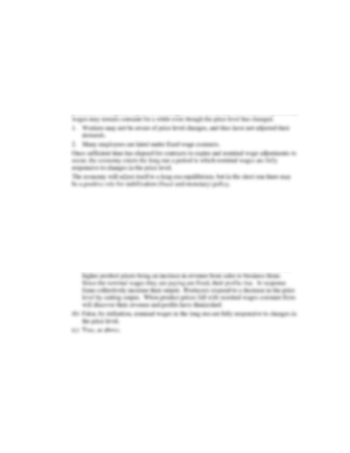
3. Suppose the full-employment level of real output (Q) for a hypothetical economy is $250 and
the price level (P) initially is 100. Use the short-run aggregate supply schedules below to answer
the questions that follow: LO1
Chapter 18 – Extending the Analysis of Aggregate Supply
18-2
a.What will be the level of real output in the short run if the price level unexpectedly rises from
100 to 125 because of an increase in aggregate demand? What if the price level unexpectedly falls
from 100 to 75 because of a decrease in aggregate demand? Explain each situation, using
numbers from the table.
b.What will be the level of real output in the long run when the price level rises from 100 to 125?
When it falls from 100 to 75? Explain each situation.
c. Show the circumstances described in parts a and b on graph paper, and derive the long-run
aggregate supply curve.
Answer:
(a) $280; $220. When the price level rises from 100 to 125 [in aggregate supply
schedule AS(P100)], producers experience higher prices for their products. Because
4. Use graphical analysis to show how each of the following would affect the economy first in
the short run and then in the long run. Assume that the United States is initially operating at its
full-employment level of output, that prices and wages are eventually flexible both upward and
downward, and that there is no counteracting fiscal or monetary policy. LO2
a.Because of a war abroad, the oil supply to the United States is disrupted, sending oil prices
rocketing upward.
b.Construction spending on new homes rises dramatically, greatly increasing total U.S.
investment spending.
c.Economic recession occurs abroad, significantly reducing foreign purchases of U.S. exports.
Answer:
(a) See Figure 35.4 in the chapter, less AD2. Short run: The aggregate supply curve
Chapter 18 – Extending the Analysis of Aggregate Supply
18-3
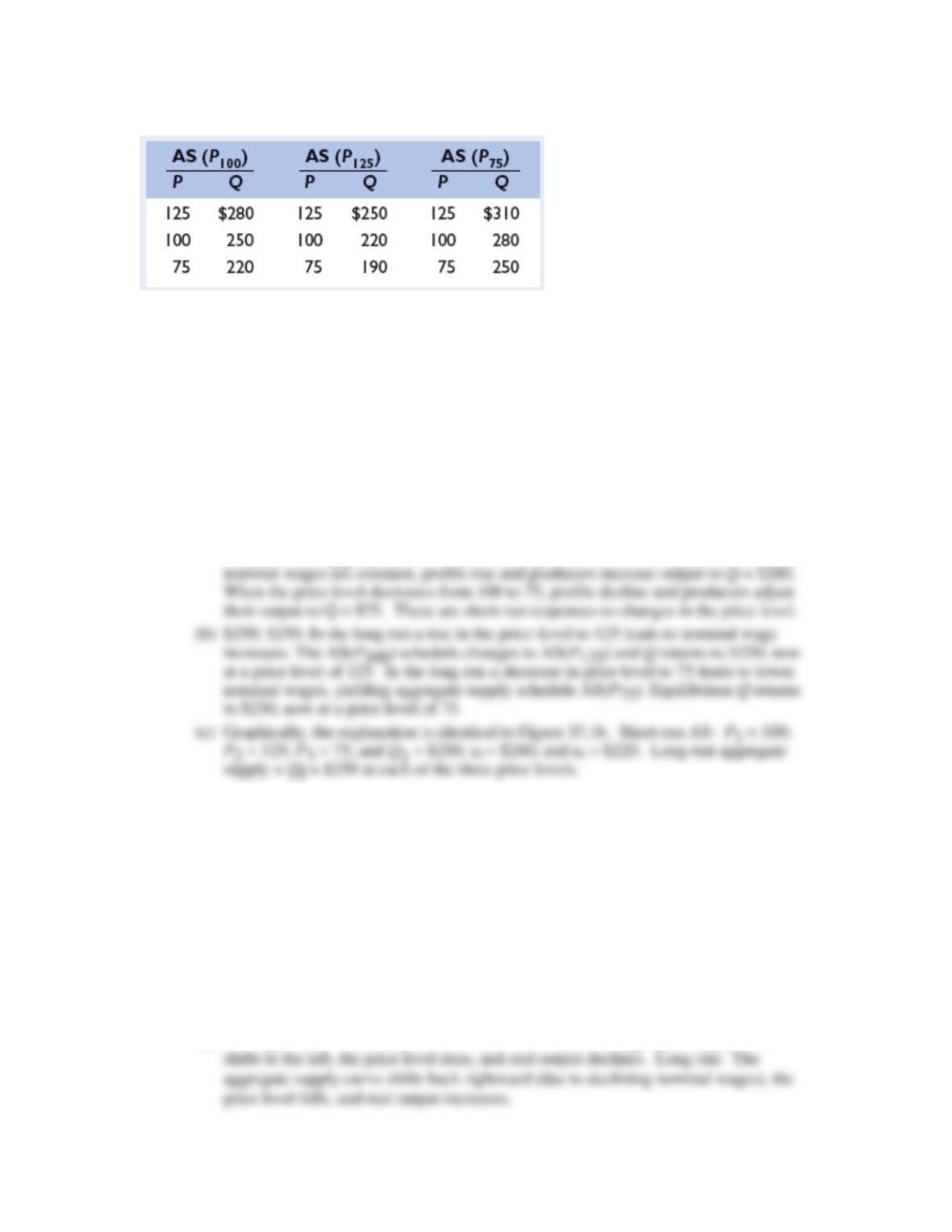
5. Between 1990 and 2009, the U.S. price level rose by about 64 percent while real output
increased by about 62 percent. Use the aggregate demand–aggregate supply model to illustrate
these outcomes graphically. LO2
Answer: In the graph shown, both AD and AS expanded over the 1990-2009 period. P2
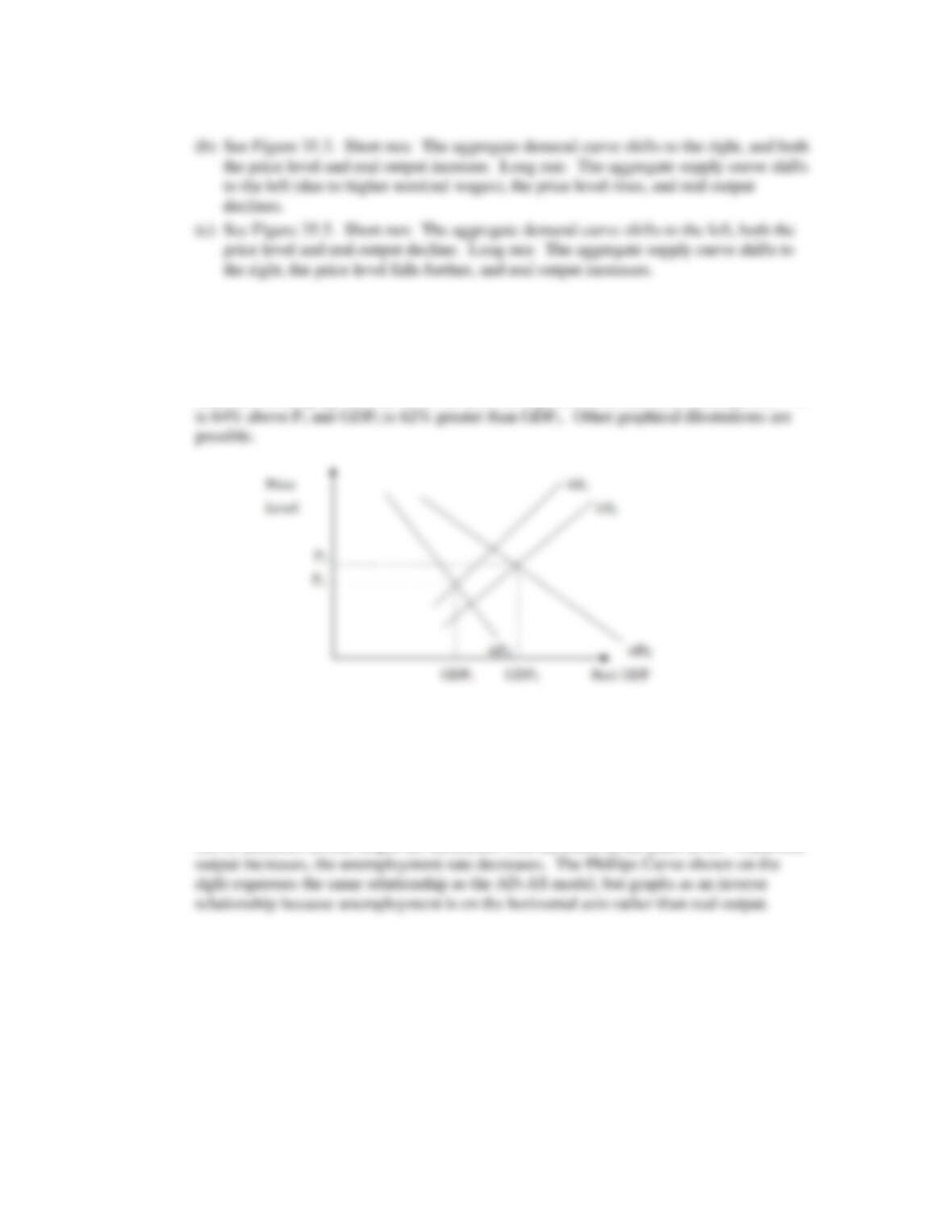
6. Assume there is a particular short-run aggregate supply curve for an economy and the curve is
relevant for -several years. Use the AD-AS analysis to show graphically why higher rates of
inflation over this period would be associated with lower rates of unemployment, and vice versa.
What is this inverse relationship called? LO3
Answer: As aggregate demand increases given a particular short-run aggregate supply
curve, increases in real output are associated with increases in the price level. When real
Chapter 18 – Extending the Analysis of Aggregate Supply
18-4
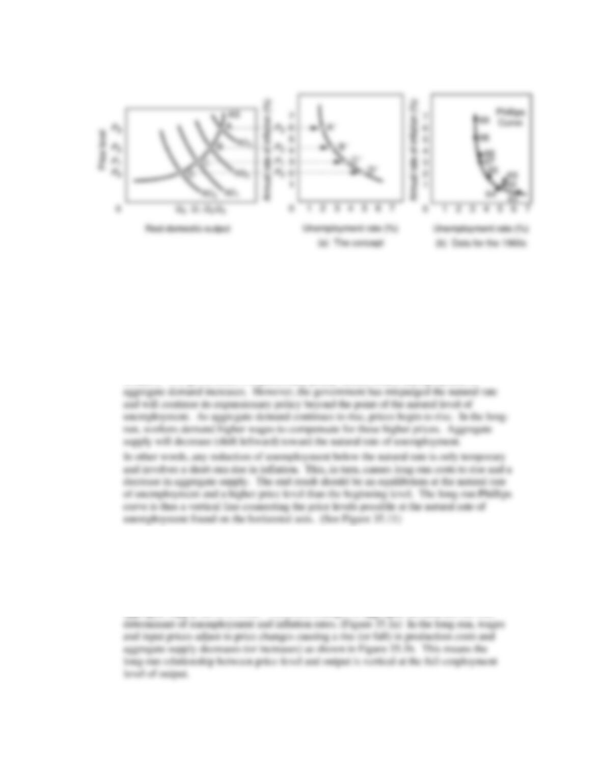
7. Suppose the government misjudges the natural rate of unemployment to be much lower than it
actually is, and thus undertakes expansionary fiscal and monetary policies to try to achieve the
lower rate. Use the concept of the short-run Phillips Curve to explain why these policies might at
first succeed. Use the concept of the long-run Phillips Curve to explain the long-run outcome of
these policies. LO4
Answer: In the short-run there is probably a tradeoff between unemployment and
inflation. The government’s expansionary policy should reduce unemployment as
8. What do the distinctions between short-run aggregate supply and long-run aggregate supply
have in common with the distinction between the short-run Phillips Curve and the long-run
Phillips Curve? Explain. LO4
Answer: In the short-run, economists assume that production costs don’t change so the
aggregate supply curve is fixed. Therefore, changes in aggregate demand are the sole
Chapter 18 – Extending the Analysis of Aggregate Supply
18-5
9. What is the Laffer Curve, and how does it relate to supply-side economics? Why is
determining the economy’s location on the curve so important in assessing tax policy? LO5
Answer: Economist Arthur Laffer observed that tax revenues would obviously be zero
when the tax rate was either at 0% or 100%. In between these two extremes would have
10. Why might one person work more, earn more, and pay more income tax when his or her tax
rate is cut, while another person will work less, earn less, and pay less income tax under the same
circumstance? LO5
Answer: Proponents of supply-side economics argue that cuts in the marginal tax rate on
earned income will make work more attractive because the opportunity cost of leisure is
11. LAST WORD On average, does an increase in taxes raise or lower real GDP? If taxes as a
percent of GDP go up 1 percent, by how much does real GDP change? Are the decreases in real
GDP caused by tax increases temporary or permanent? Does the intention of a tax increase
matter?
Answer: C. Romer and D. Romer show that tax increases reduce real GDP. On average
a 1 percent tax increase (as percentage of real GDP) reduces real GDP by 2 to 3 percent.
Chapter 18 – Extending the Analysis of Aggregate Supply
18-6
PROBLEMS
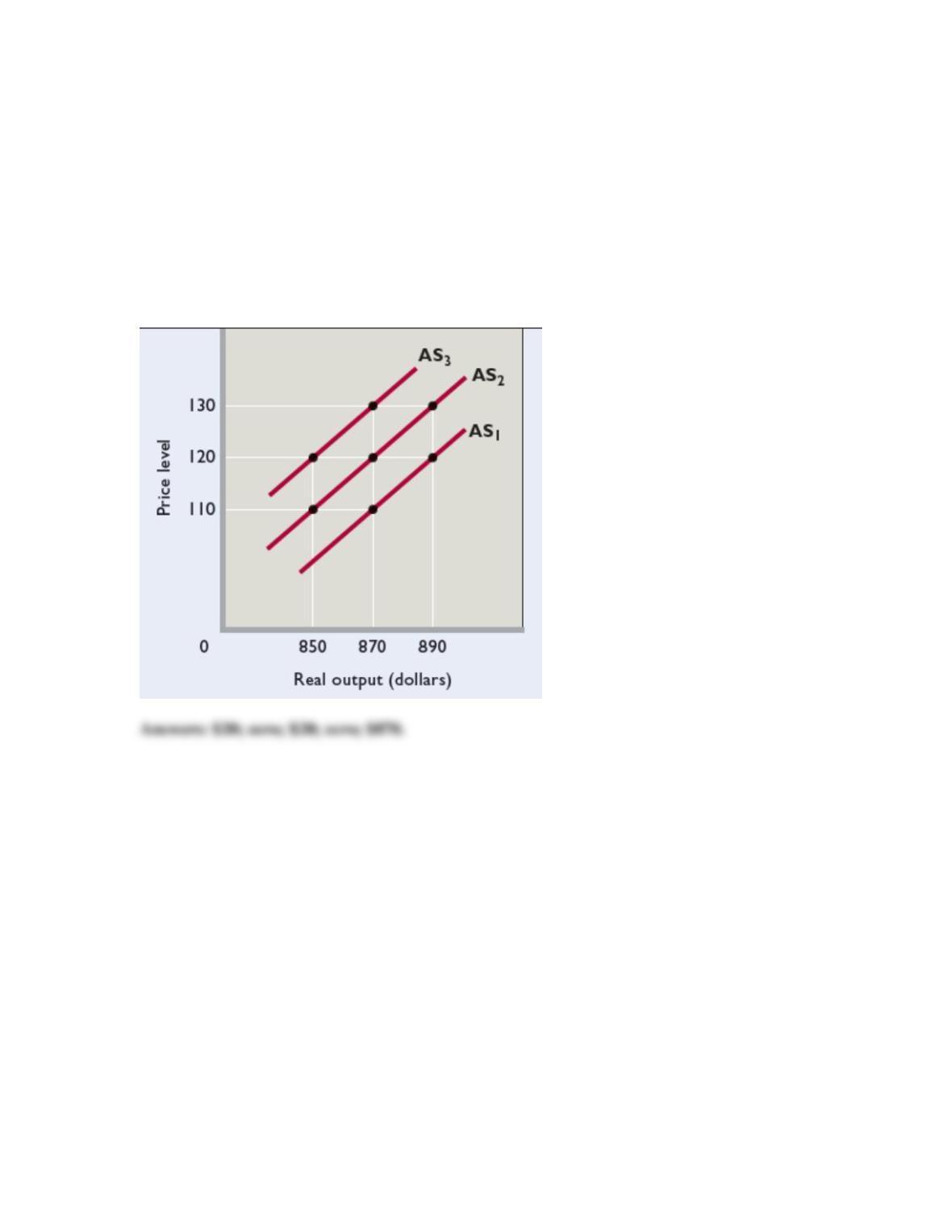
1. Use the accompanying figure to answer the follow questions. Assume that the economy
initially is operating at price level 120 and real output level $870. This output level is the
economy’s potential (or full-employment) level of output. Next, suppose that the price level rises
from 120 to 130. By how much will real output increase in the short run? In the long-run?
Instead, now assume that the price level dropped from 120 to 110. Assuming flexible product and
resource prices, by how much will real output fall in the short run? In the long run? What is the
long-run level of output at each of the three price levels shown?
LO1
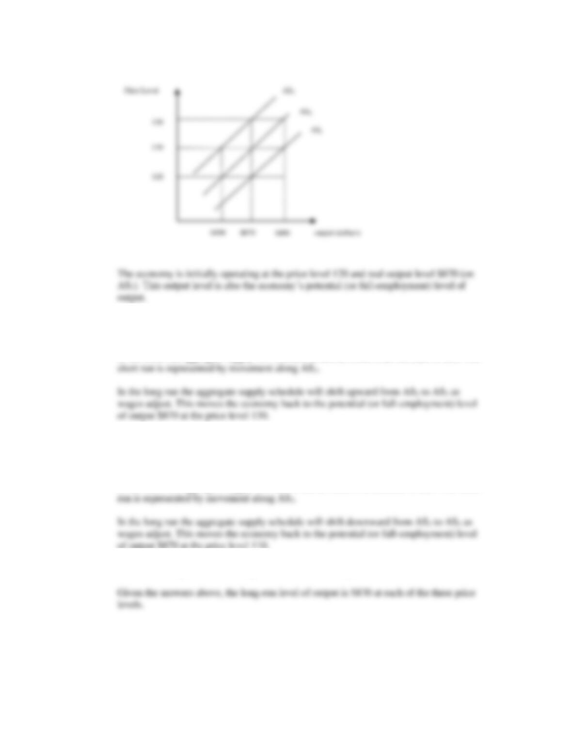
Feedback: Consider the following example. Use the accompanying figure to answer the
follow questions. Assume that the economy initially is operating at price level 120 and
real output level $870. This output level is the economy’s potential (or full-employment)
level of output. Next, suppose that the price level rises from 120 to 130. By how much
will real output increase in the short run? In the long-run? Instead, now assume that the
price level dropped from 120 to 110. Assuming flexible product and resource prices, by
how much will real output fall in the short run? In the long run? What is the long-run
level of output at each of the three price levels shown?
Chapter 18 – Extending the Analysis of Aggregate Supply
18-7
Next, suppose that the price level rises from 120 to 130. By how much will real output
increase in the short run? In the long-run?
In the short run aggregate supply will increase to $890, which is an increase of $20. The
Instead, now assume that the price level dropped from 120 to 110. Assuming flexible
product and resource prices, by how much will real output fall in the short run? In the
long run?
In the short run aggregate supply will fall to $850, which is a decrease of $20. The short
of output $870 at the price level 110.
What is the long-run level of output at each of the three price levels shown?
Chapter 18 – Extending the Analysis of Aggregate Supply
18-8
2. ADVANCED ANALYSIS Suppose that the equation for a particular short-run AS curve is P
= 20 + .5Q, where P is the price level and Q is real output in dollar terms. What is Q if the price
level is 120? Suppose that the Q in your answer is the full-employment level of output. By how
much will Q increase in the short run if the price level unexpectedly rises from 120 to 132? By
how much will Q increase in the long-run due to the price level increase? LO1
Feedback: Consider the following example. Suppose that the equation for a particular
short-run AS curve is P = 20 + .5Q, where P is the price level and Q is real output in
dollar terms. What is Q if the price level is 120? Suppose that the Q in your answer is the
full-employment level of output. By how much will Q increase in the short run if the
price level unexpectedly rises from 120 to 132? By how much will Q increase in the
long-run due to the price level increase?
Since we are given the price level we need to solve the short-run AS curve for Q as a
function of P.
3. Suppose that over a 30-year period Buskerville’s price level increased from 72 to 138 while its
real GDP rose from $1.2 trillion to $2.1 trillion. Did economic growth occur in Buskerville? If so,
by what average yearly rate? Did Buskerville experience inflation? If so, by what average yearly
rate? Which shifted rightward faster in Buskerville: its long-run aggregate supply curve (ASLR)
or its aggregate demand curve (AD)? LO2
Chapter 18 – Extending the Analysis of Aggregate Supply
18-9
Feedback: Consider the following example. Suppose that over a 30-year period
Buskerville’s price level increased from 72 to 138 while its real GDP rose from $1.2
trillion to $2.1 trillion. Did economic growth occur in Buskerville? If so, by what average
yearly rate? Did Buskerville experience inflation? If so, by what average yearly rate?
Which shifted rightward faster in Buskerville: its long-run aggregate supply curve
(ASLR) or its aggregate demand curve (AD)?
Did economic growth occur in Buskerville?
If so, by what average yearly rate?
First, find the rate of growth for the given period of time (30 year period in this example).
Did Buskerville experience inflation?
If so, by what average yearly rate?
First, find the inflation rate for the given period of time (30 year period in this example).
Which shifted rightward faster in Buskerville: its long-run aggregate supply curve
(ASLR) or its aggregate demand curve (AD)?
4. Suppose that for years East Confetti’s short-run Phillips Curve was such that each 1 percentage
point increase in its unemployment rate was associated with a 2 percentage point decline in its
inflation rate. Then, during several recent years the short run pattern changed such that its
inflation rate rose by 3 percentage points for every 1 percentage point drop in its unemployment
rate. Graphically, did East Confetti’s Phillips Curve shift upward or did it shift downward? LO3
Chapter 18 – Extending the Analysis of Aggregate Supply
18–10
Feedback: Consider the following example. Suppose that for years East Confetti’s short–
run Phillips Curve was such that each 1 percentage point increase in its unemployment
rate was associated with a 2 percentage point decline in its inflation rate. Then, during
several recent years the short run pattern changed such that its inflation rate rose by 3
percentage points for every 1 percentage point drop in its unemployment rate.
Graphically, did East Confetti’s Phillips Curve shift upward or did it shift downward?
The answer is upward.