Economics Chapter 17 The Model Can Estimated Ols Maximum Likelihood

CHAPTER 17

TEACHING NOTES

I emphasize to the students that, first and foremost, the reason we use the probit and logit models

is to obtain more reasonable functional forms for the response probability. Once we move to a

nonlinear model with a fully specified conditional distribution, it makes sense to use the efficient

estimation procedure, maximum likelihood. It is important to spend some time on interpreting

probit and logit estimates. In particular, the students should know the rules-of-thumb for

I view the Tobit model, when properly applied, as improving functional form for corner solution

outcomes. (I believe this motivated Tobin’s original work, too.) In most cases, it is wrong to

view a Tobit application as a data-censoring problem (unless there is true data censoring in

collecting the data or because of institutional constraints). For example, in using survey data to

estimate the demand for a new product, say a safer pesticide to be used in farming, some farmers

Poisson regression with an exponential conditional mean is used primarily to improve over a

linear functional form for E(y|x) for count data. The parameters are easy to interpret as semi-

elasticities or elasticities. If the Poisson distributional assumption is correct, we can use the

Poisson distribution to compute probabilities, too. Unfortunately, overdispersion is often present

220

on censored and truncated regression. In fact, I put the Poisson regression model between these

two topics on purpose: I hope it emphasizes that the material in Section 17.2 is purely about

functional form, as is Poisson regression. Sections 17.4 and 17.5 deal with underlying linear

models, but where there is a data-observability problem.

221

SOLUTIONS TO PROBLEMS

17.1 (i) Let m0 denote the number (not the percent) correctly predicted when yi = 0 (so the

prediction is also zero) and let m1 be the number correctly predicted when yi = 1. Then the

(ii) We just use the formula from part (i):

ˆ

p

= .30(80) + .70(40) = 52. Therefore, overall we

17.2 We need to compute the estimated probability first at hsGPA = 3.0, SAT = 1,200, and

study = 10 and subtract this from the estimated probability with hsGPA = 3.0, SAT = 1,200, and

study = 5. To obtain the first probability, we start by computing the linear function inside ():

17.3 (i) We use the chain rule and equation (17.23). In particular, let x1  log(z1). Then, by the

chain rule,

E(y|y > 0,x)/ x1, we obtain the answer.

(ii) As in part (i), we use the chain rule, which is now more complicated:

17.4 Since log() is an increasing function – that is, for positive w1 and w2, w1 > w2 if and only if

17.5 (i) patents is a count variable, and so the Poisson regression model is appropriate.

(ii) Because



1 is the coefficient on log(sales),



1 is the elasticity of patents with respect to

sales. (More precisely,



1 is the elasticity of E(patents|sales,RD) with respect to sales.)

17.6 (i) OLS will be unbiased, because we are choosing the sample on the basis of an exogenous

explanatory variable. The population regression function for sav is the same as the regression

function in the subpopulation with age > 25.

(ii) Assuming that marital status and number of children affect sav only through household

223

17.7 For the immediate purpose of determining the variables that explain whether accepted

applicants choose to enroll, there is not a sample selection problem. The population of interest is

applicants accepted by the particular university, and you have a random sample from this

population. Therefore, it is perfectly appropriate to specify a model for this group, probably a

SOLUTIONS TO COMPUTER EXERCISES

C17.1 (i) If spread is zero, there is no favorite, and the probability that the team we (arbitrarily)

label the favorite should have a 50% chance of winning.

(ii) The linear probability model estimated by OLS gives

(iii) As we expect, spread is very statistically significant using either standard error, with a t

224

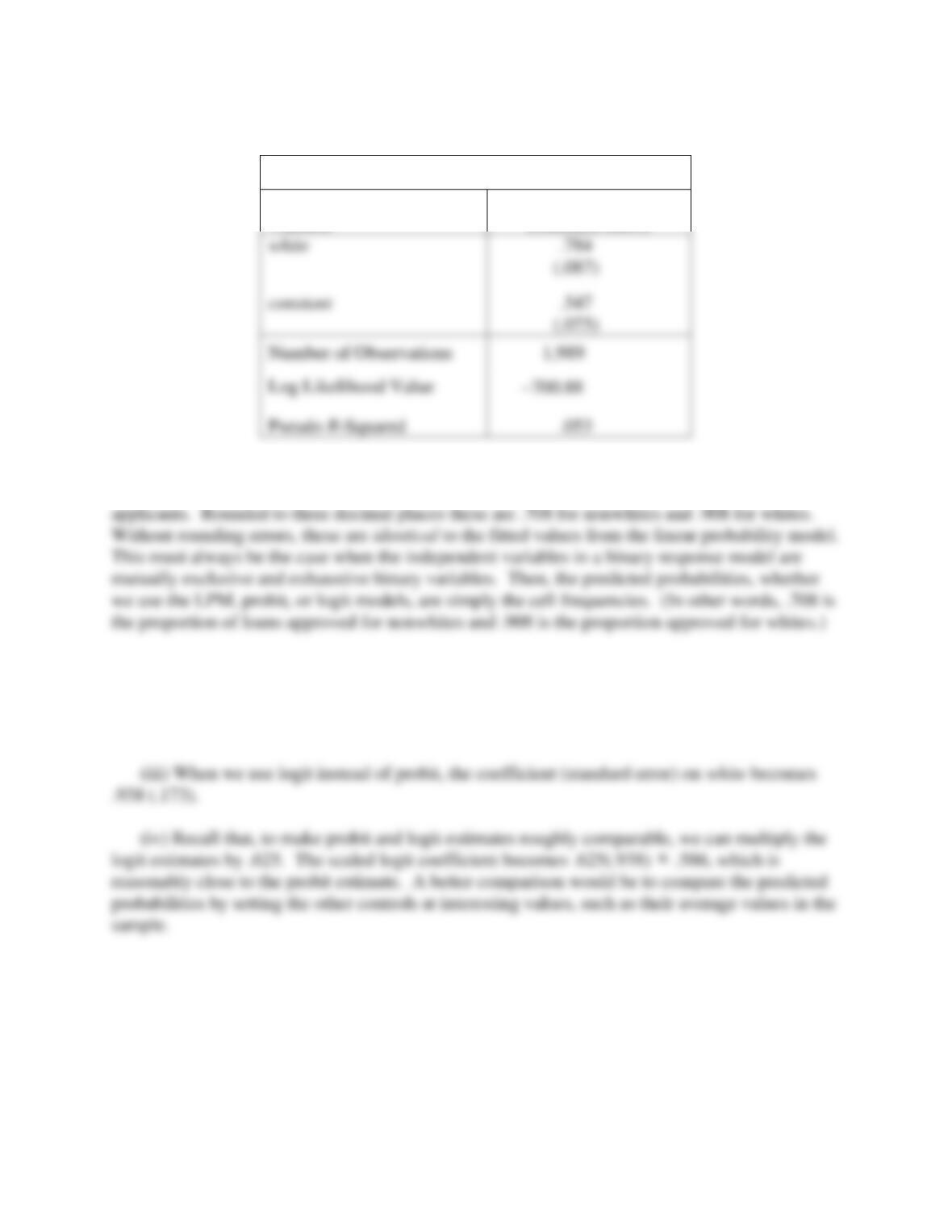
(iv) The probit results are given in the following table:

Dependent Variable: favwin

where () denotes the standard normal cdf, if



0 = 0 then

(vi) When favhome, fav25, and und25 are added to the probit model, the value of the log-

likelihood becomes –262.64. Therefore, the likelihood ratio statistic is 2[−262.64 – (−263.56)] =

Number of Observations

Log Likelihood Value

Pseudo R-Squared

225

C17.2 (i) The probit estimates from approve on white are given in the following table:

Dependent Variable: approve

Independent

Variable

Coefficient

(Standard Error)

As there is only one explanatory variable that takes on just two values, there are only two

different predicted values: the estimated probabilities of loan approval for white and nonwhite

(ii) With the set of controls added, the probit estimate on white becomes about .520 (se



.097). Therefore, there is still very strong evidence of discrimination against nonwhites. We can

divide this by 2.5 to make it roughly comparable to the LPM estimate in part (iii) of Computer

Exercise C7.8: .520/2.5



.208, compared with .129 in the LPM.

C17.3 (i) Out of 616 workers, 172, or about 18%, have zero pension benefits. For the 444

workers reporting positive pension benefits, the range is from $7.28 to $2,880.27. Therefore, we

have a nontrivial fraction of the sample with pensiont = 0, and the range of positive pension

benefits is fairly wide. The Tobit model is well-suited to this kind of dependent variable.

(ii) The Tobit results are given in the following table:

Number of Observations

1,989

Log Likelihood Value

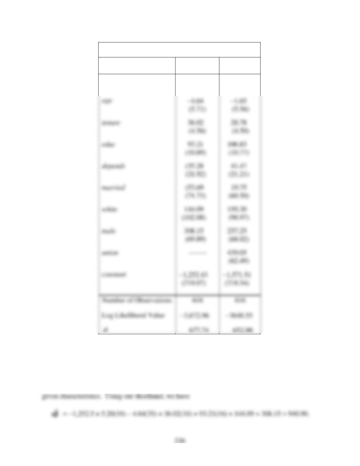
Dependent Variable: pension

Independent

Variable

(1)

(2)

exper

5.20

(6.01)

4.39

(5.83)

tenure

educ

married

white

union

In column (1), which does not control for union, being white or male (or, of course, both)

increases predicted pension benefits, although only male is statistically significant (t



4.41).

(iii) We use equation (17.22) with exper = tenure = 10, age = 35, educ = 16, depends = 0,

married = 0, white = 1, and male = 1 to estimate the expected benefit for a white male with the

227

Therefore, with

ˆ



= 677.74 we estimate E(pension|x) as

The difference between the white male and nonwhite female is 966.40 – 582.10 = $384.30.

[Instructor’s Note: If we had just done a linear regression, we would add the coefficients on

white and male to obtain the estimated difference. We get about 114.94 + 272.95 = 387.89,

which is very close to the Tobit estimate. Provided that we focus on partial effects, Tobit and a

linear model can give similar answers for explanatory variables near the mean values.]

228

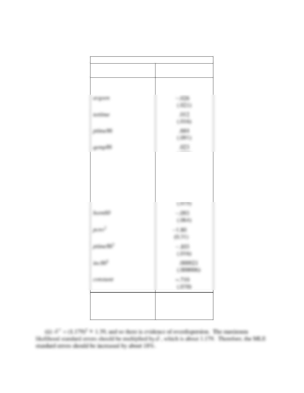
C17.4 (i) The results for the Poisson regression model that includes pcnv2, ptime862, and inc862

are given in the following table:

Dependent Variable: narr86

Independent

Variable

Coefficient

(Standard Error)

pcnv

1.15

(0.28)

(.033)

inc86

−.012

(.002)

black

.591

(.074)

hispan

born60

−.093

(.064)

−.103

(.000006)

.422

Number of Observations

2,725

Log Likelihood Value

−2,168.87

ˆ



1.179

avgsen

−.026

(.021)

ptime86

(.091)

qemp86

229

(iii) From Table 17.3 we have the log-likelihood value for the restricted model, Lr =

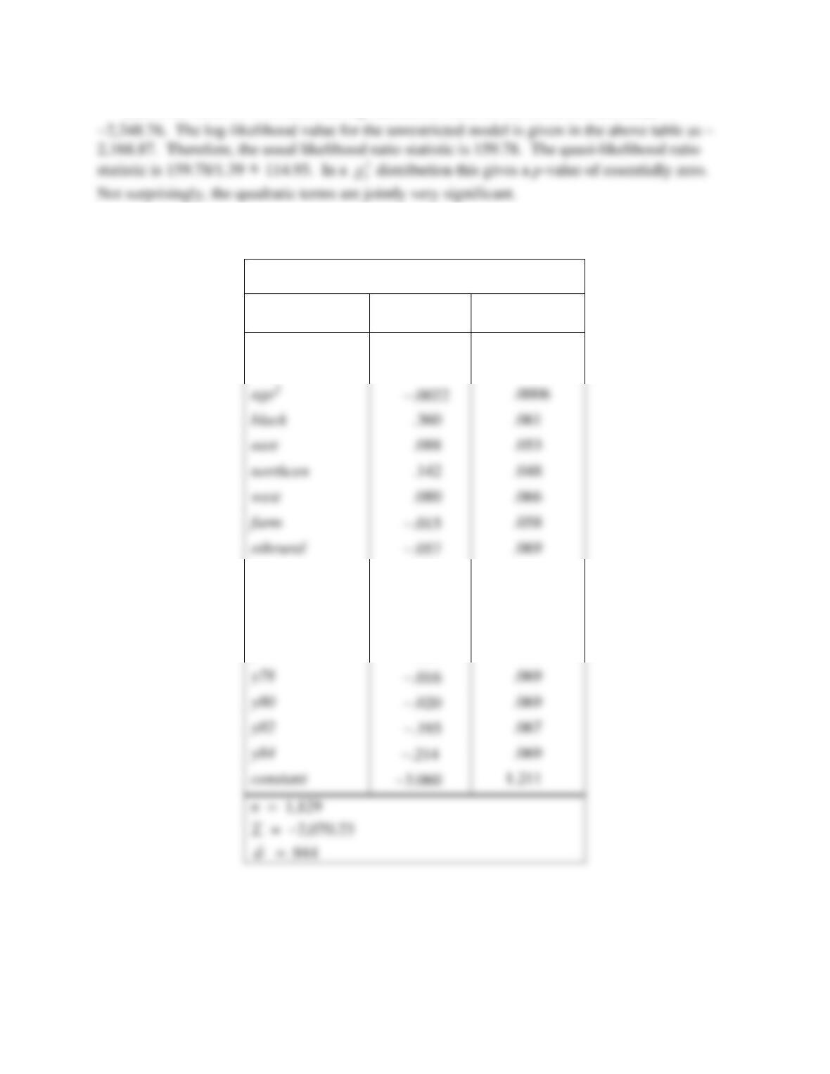
C17.5 (i) The Poisson regression results are given in the following table:

Dependent Variable: kids

Independent

Variable

Coefficient

Standard

Error

educ

−.048

.007

age

.204

.055

−.0022

.0006

black

.360

.061

east

.088

.053

northcen

.142

.048

west

.080

.066

farm

−.015

.058

town

.031

.049

smcity

.074

.062

y74

.093

.063

y76

−.029

.068

y78

−.016

.069

y80

.069

y82

−.193

.067

y84

.069

The coefficient on y82 means that, other factors in the model fixed, a woman’s fertility was

about 19.3% lower in 1982 than in 1972.

230

(ii) Because the coefficient on black is so large, we obtain the estimated proportionate

difference as exp(.36) – 1



.433, so a black woman has 43.3% more children than a comparable

nonblack woman. (Notice also that black is very statistically significant.)