Economics Chapter 17 Several new time series data sets include OKUN

231

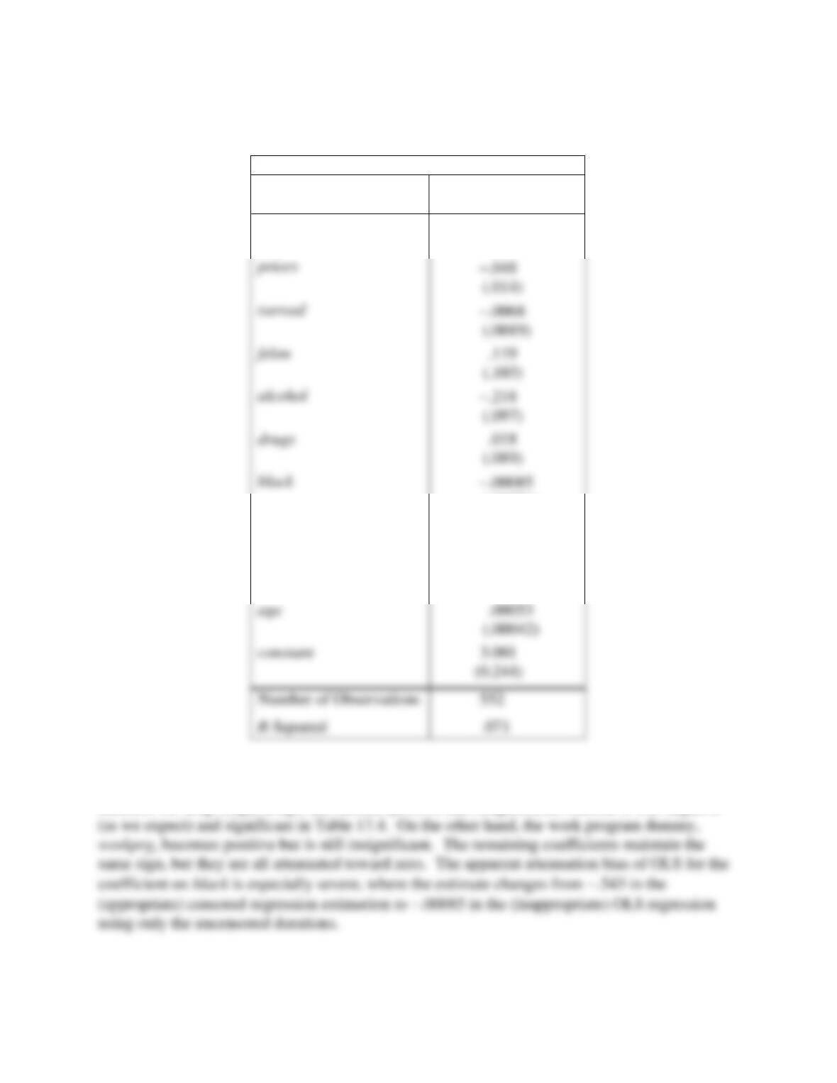
C17.6 The results of an OLS regression using only the uncensored durations are given in the

following table:

Dependent Variable: log(durat)

Independent

Variable

Coefficient

(Standard Error)

workprg

.092

(.083)

(.08221)

married

.239

(.099)

educ

−.019

(.019)

age

.00053

(.00042)

There are several important differences between the OLS estimates using the uncensored

durations and the estimates from the censored regression in Table 17.4. For example, the binary

indicator for drug usage, drugs, has become positive and insignificant, whereas it was negative

(.014)

felon

.119

(.103)

alcohol

−.218

(.097)

drugs

.018

(.089)

232

C17.7 (i) When log(wage) is regressed on educ, exper, exper2, nwifeinc, age, kidslt6, and

kidsge6, the coefficient and standard error on educ are .0999 (se = .0151).

(ii) The Heckit coefficient on educ is .1187 (se = .0341), where the standard error is just the

C17.8 (i) 185 out of 445 participated in the job training program. The longest time in the

experiment was 24 months (obtained from the variable mosinex).

(ii) The F statistic for joint significance of the explanatory variables is F(7,437) = 1.43 with

usual F statistic is asymptotically valid.

(iii) After estimating the model P(train = 1|x) = (



0 +



1unem74 +



2unem75 +



3age +

(iv) Training eligibility was randomly assigned among the participants, so it is not surprising

that train appears to be independent of other observed factors. (However, there can be a

difference between eligibility and actual participation, as men can always refuse to participate if

chosen.)

(v) The simple LPM results are

233

the regression is very small. There is much about being unemployed that we are not explaining,

but we can be pretty confident that this job training program was beneficial.)

(vi) The estimated probit model is

(vii) There are only two fitted values in each case, and they are the same: .354 when train =

0 and .243 when train = 1. This has to be the case, because any method simply delivers the cell

frequencies as the estimated probabilities. The LPM estimates are easier to interpret because

they do not involve the transformation by (), but it does not matter which is used provided the

probability differences are calculated.

(viii) The fitted values are no longer identical because the model is not saturated, that is, the

(ix) To obtain the average partial effect of train using the probit model, we obtain fitted

probabilities for each man for train = 1 and train = 0. Of course, on of these is a counterfactual,

C17.9 (i) 248.

(ii) The distribution is not continuous: there are clear focal points, and rounding. For

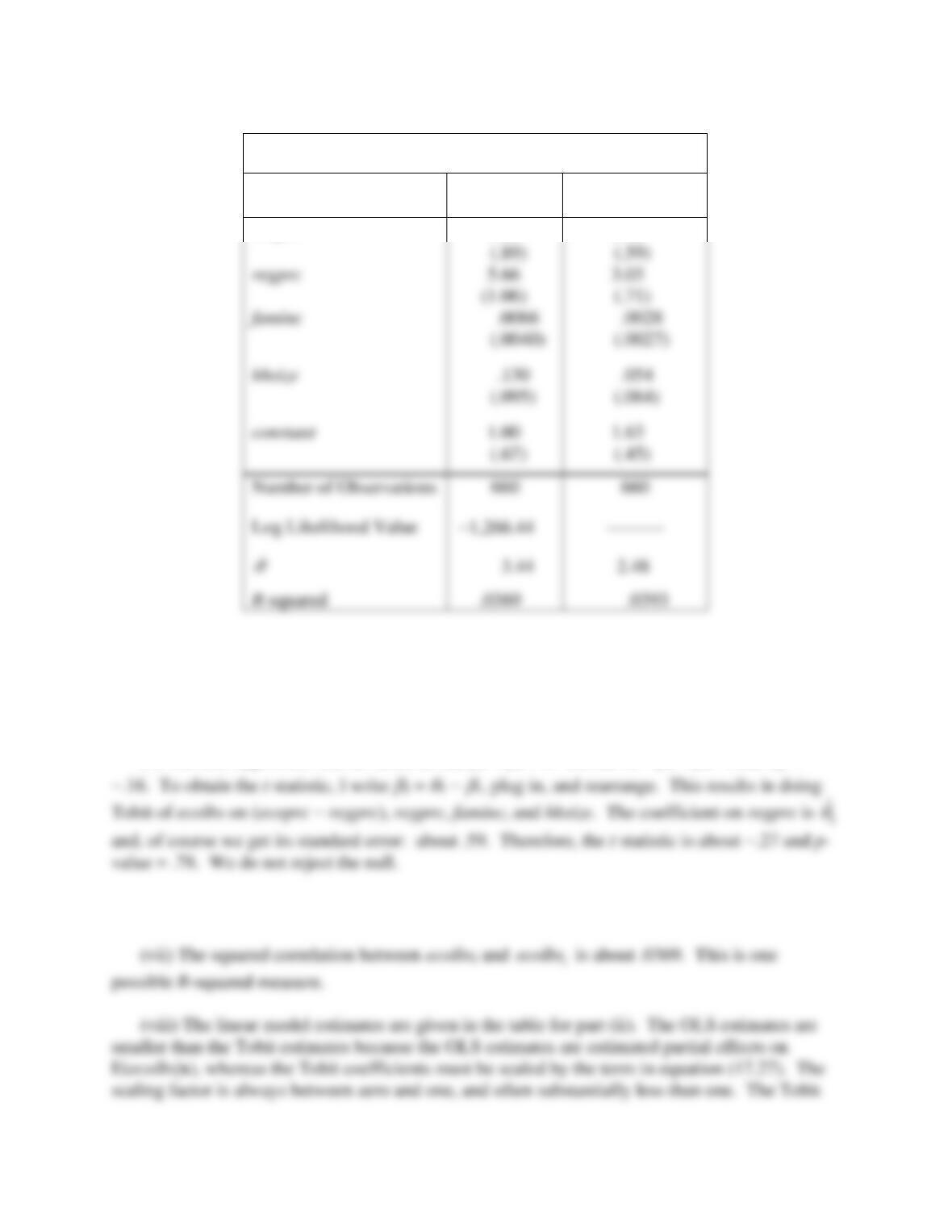
(ii) The following table contains the Tobit estimates and, for later comparison, OLS

estimates of a linear model:

234

Dependent Variable: ecolbs

Independent

Variable

Tobit

OLS

(Linear Model)

ecoprc

−5.82

−2.90

Only the price variables, ecoprc and regprc, are statistically significant at the 1% level.

(iv) The signs of the price coefficients accord with basic demand theory: the own-price

effect is negative, the cross price effect for the substitute good (regular apples) is positive.

(v) The null hypothesis can be stated as H0:



1 +



2 = 0. Define



1 =



1 +



2. Then

1

ˆ



=

(vi) The smallest fitted value is .798, while the largest is 3.327.

model does not fit better, at least in terms of estimating E(ecolbs|x): the linear model R-squared

is a bit larger (.0393 versus .0369).

(ix) This is not a correct statement. We have another case where we have confidence in the

C17.10 (i) 497 people do not smoke at all. 101 people report smoking 20 cigarettes a day. Since

one pack of cigarettes contains 20 cigarettes, it is not surprising that 20 is a focal point.

(ii) The Poisson distribution does not allow for the kinds of focal points that characterize

cigs. If you look at the full frequency distribution, there are blips at half a pack, two packs, and

236

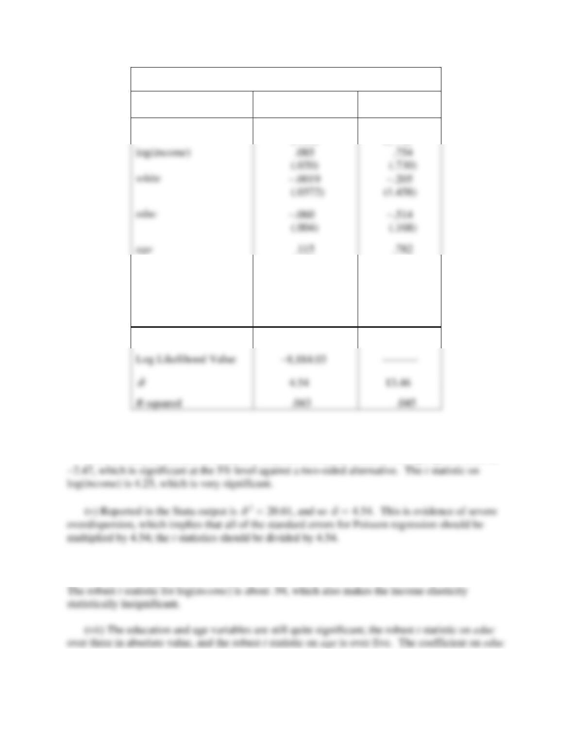
Dependent Variable: cigs

Independent

Variable

Poisson

(Exponential Model)

OLS

(Linear Model)

log(cigpric)

−.355

(.144)

−2.90

(5.70)

(.005)

(.161)

age2

−.00138

(.00006)

−.0091

(.0018)

constant

1.46

(.61)

5.77

(24.08)

Number of Observations

807

The estimated price elasticity is −.355 and the estimated income elasticity is .085.

(iv) If we use the maximum likelihood standard errors, the t statistic on log(cigpric) is about

(vi) The robust t statistic for log(cigpric) is about −.54, which makes it very insignificant.

This is a good example of misleading the usual Poisson standard errors and test statistics can be.

(.020)

(.730)

237

implies that one more year of education reduces the expected number of cigarettes smoked by

about 6.0%.

(viii) The minimum predicted value is .515 and the maximum is 18.84. The fact that we

(ix) The squared correlation between cigsi and

i

cigs

is the R-squared reported in the above

table, .043.

(x) The linear model results are reported in the last column of the previous table. The R–

C17.11 (i) The fraction of women in the work force is 3,286/5,634  .583.

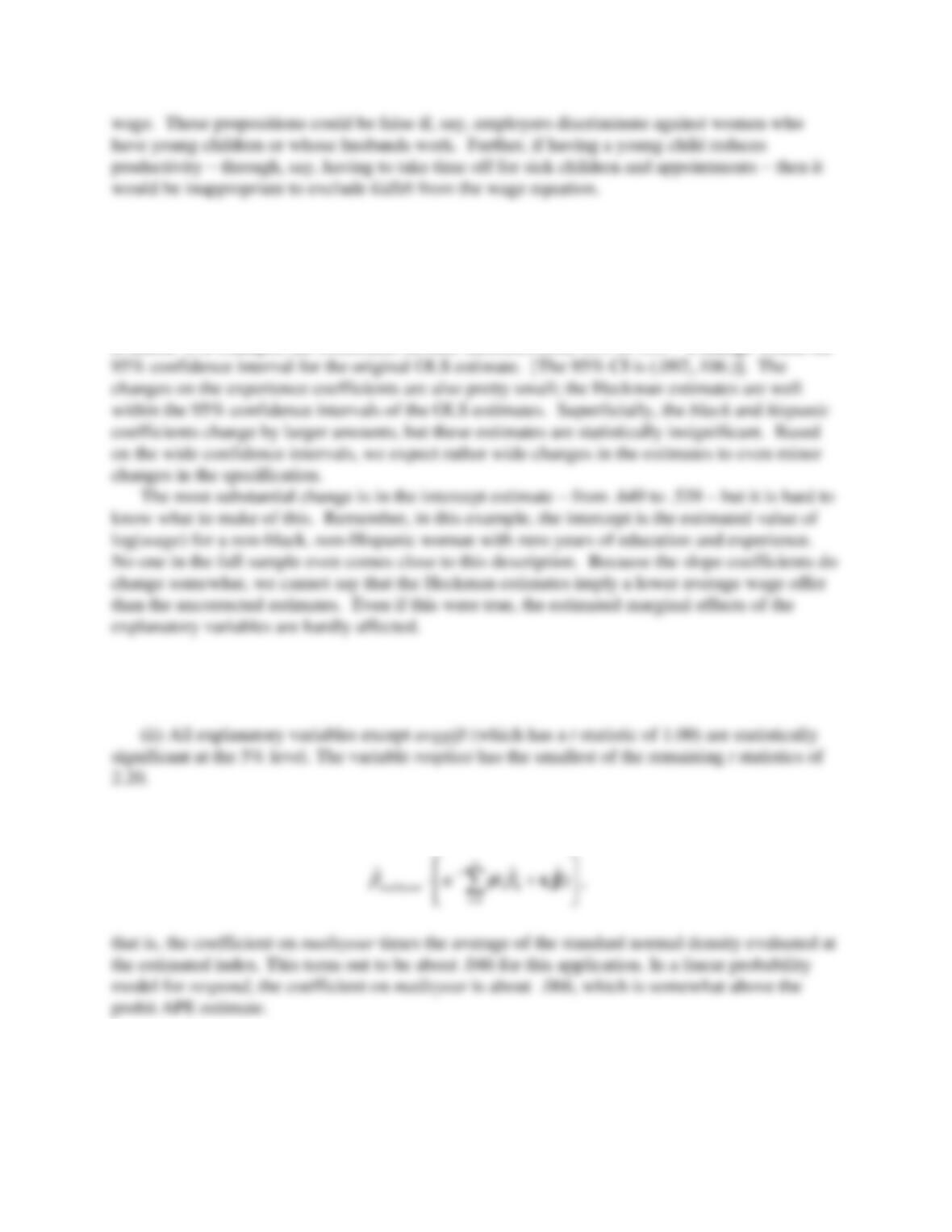
(ii) The OLS results using the selected sample are

(iii) The coefficient on nwifeinc is −.0091 with t = −13.47 and the coefficient on kidlt6 is

−.500 with t = −11.05. We expect both coefficients to be negative. If a woman’s spouse earns

(iv) We need at least one variable to affect labor force participation that does not have a

direct effect on the wage offer. So, we must assume that, controlling for education, experience,

and the race/ethnicity variables, other income and the presence of a young children do not affect

238

(v) The t statistic on the inverse Mills ratio is 1.77 and the p-value against the two-sided

alternative is .077. With 3,286 observations, this is not a very small p-value. The test on

ˆ



does

not provide strong evidence against the null hypothesis of no selection bias.

(vi) Just as important, the slope coefficients do not change much when the inverse Mills ratio

is added. For example, the coefficient on educ increases from .099 to .103 – a change within the

C17.12 (i) Out of 4,248 respondents, 1,707 made a gift most recently. This is 40 percent of the

sample.

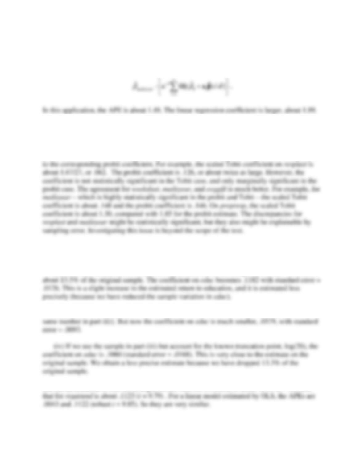
(iii) The average partial effect for mailsyear is

(iv) In the Tobit estimation, all explanatory variables except replast are strongly statistically

significant. The t statistic on replast is 1.24. The smallest t statistic on the other variables (in

absolute value) is on avggift, 5.09.

239

(v) The APE in the Tobit case, again treating mailsyear as a continuous variable, is estimated

as

(vi) They are not entirely compatible with the Tobit model, although it is difficult to know

whether the differences are important. Subject to sampling error, the coefficients from the probit,

say

ˆj



, should be roughly equal to

ˆˆ

/

j



, where the latter are from Tobit. Now, the signs of the

probit and Tobit coefficients are all the same, but the scaled Tobit coefficient is not always close

C17.13 (i) Using the entire sample, the estimated coefficient on educ is .1037 with standard error

= .0097.

(ii) 166 observations are lost when we restrict attention to the sample with educ < 16. This is

(iii) If we restrict attention to those with wage < 20, we lose 164 observations [about the

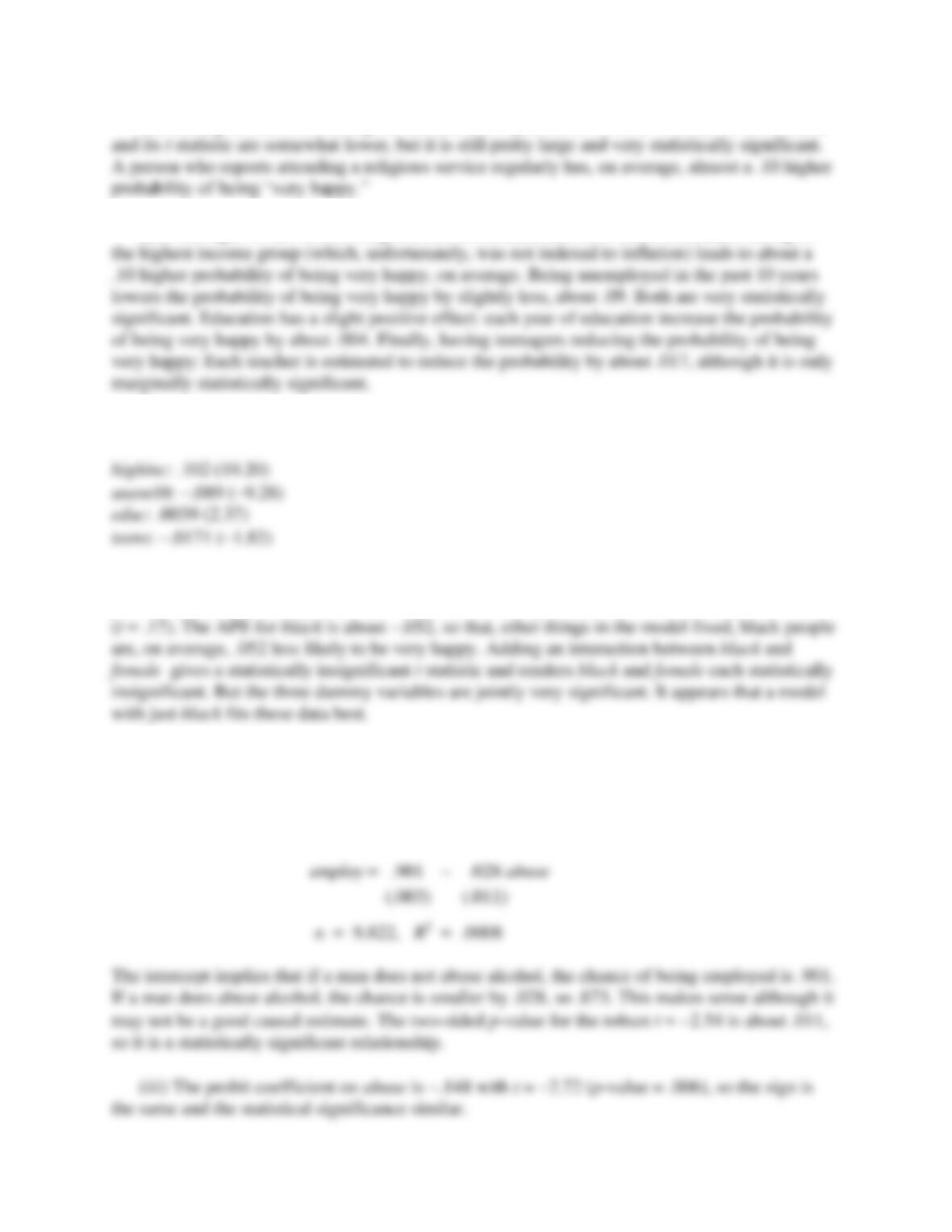
C17.14 (i) Rounded to four decimal places, the APE for occattend is about .0043 (t = .53) and

240

(ii) Adding the extra controls gives an APE for regattend of .0960 (t = 6.49). So the estimate

(iii) The signs of the APEs of highinc, unem10, educ, and teens seem reasonable. Being in

APE (t statistic):

(iv) The only race variable in the data set is the binary variable black. If we add black and

female to the probit from part (ii), black is statistically significant (t = −3.71) while female is not

C17.15 (i) The fraction of men employed is about .898 and the fraction abusing alcohol is about

.099.

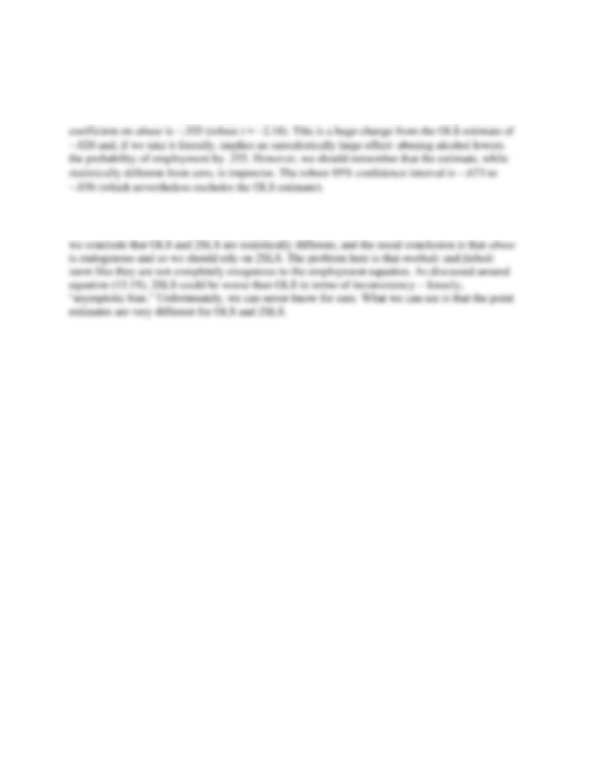
(ii) The simple regression, with heteroskedasticity-robust standard errors, is

241

(iv) The fitted values from the LPM and probit must be the same. In each case, there are only

(v) I will not report the full results here, but only what happens to the abuse coefficient. With

(vi) Estimating a probit model with the same explanatory variables from (v) and computing

the APE for abuse gives an APE of about −.021. It is no longer identical to the OLS estimate in

the linear model because the model with many covariates is not saturated. But it is close. The

probit estimate is somewhat more statistically significant with t = −1.98.

(vii) It is not clear that other health indicators should be controlled for. If they are included, it

(viii) The indicator of alcohol abuse may be correlated with unobserved factors that affect

employment. Certain kinds of health issues were already mentioned in part (vii). Depression and

low self-esteem, not being motivated are other examples. Indicators for whether one’s parents

242

So mothalc and fathalc are significant predictors of abuse, and the signs of the two coefficients

make sense.

(ix) When we use mothalc and fathalc as IVs for abuse and estimate the LPM by 2SLS, the

(x) We need to obtain the residuals,

2

ˆ

v

, from the reduced form regression. When we add the

residuals to the linear model estimated in part (v), its coefficient is .336 (robust t = 2.20). Thus,