Basic Econometrics, Gujarati and Porter
CHAPTER 17:
DYNAMIC ECONOMETRIC MODELS:
AUTOREGRESSIVE AND DISTRIBUTED-LAG MODELS
17.1 (a) False. Econometric models are dynamic if they portray
the time path of the dependent variable in relation to its past values.
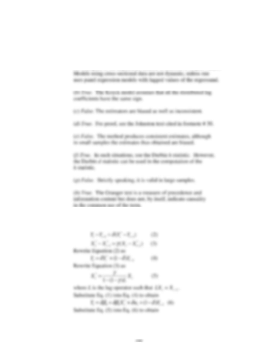
17.2 Make use of Equations (17.7.1), (17.6.2), and (17.5.2).
* *
0 1
(1)
t t t
Y X u
β β
= + +
17.3
1 1 1 1 1
cov[ ,( )] {[( ( )][ ]}
t t t t t t t
Y u u E Y E Y u u
λ λ
− − − − −
− = − −
, since
( ) 0
t
E u
=
.
P
17.5
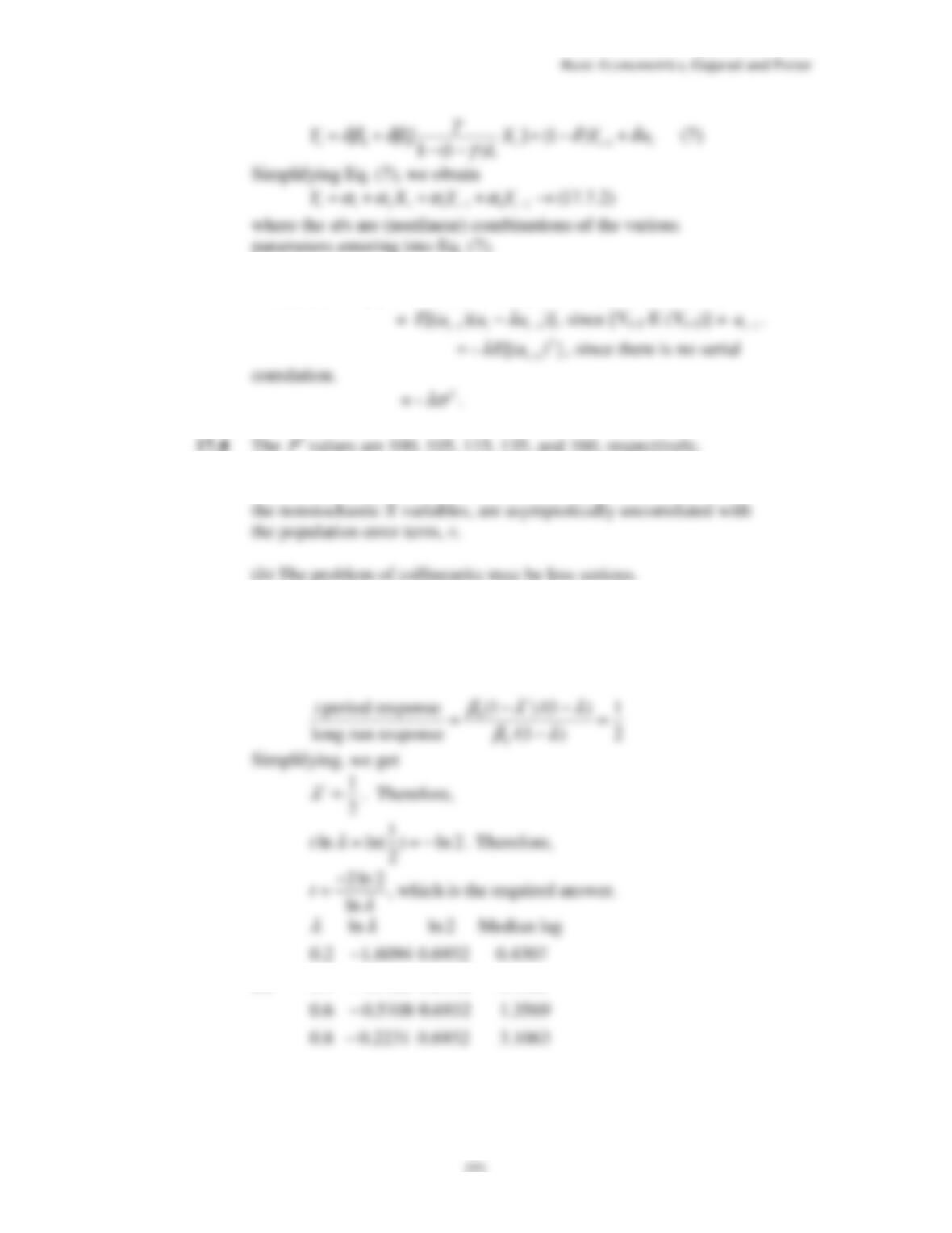
(a) The estimated Y values, which are a linear function of the
17.6
(a) The median lag is the value of time for which the fraction of
adjustment completed is ½. To find the median lag for the Koyck
scheme, solve
(b)
0.4 0.9163 0.6932 0.7565
−
17.7
(a)
Since
0
;0 1; 0,1, 2…
k
k
k
β β λ λ
= < < =
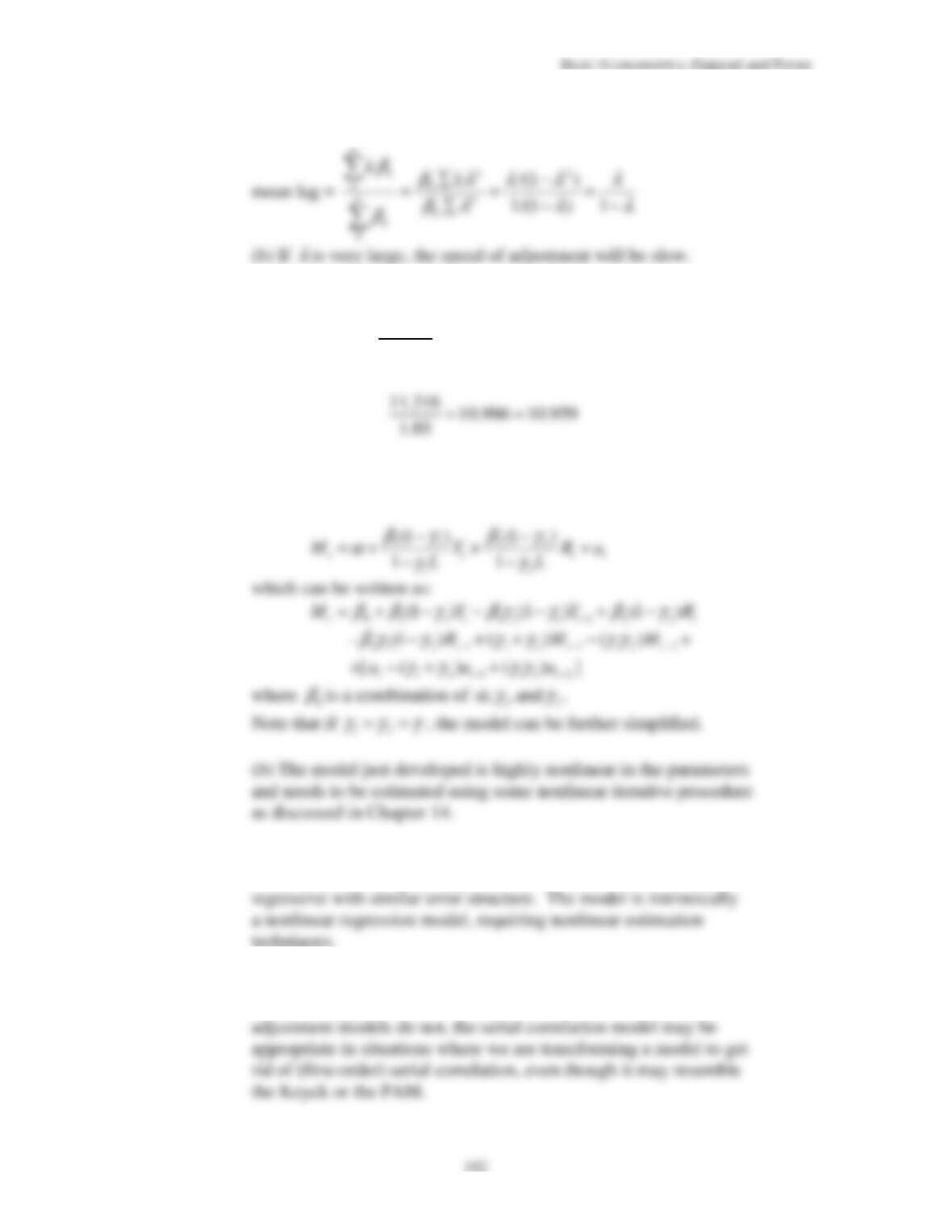
17.8 Use the formula
k
k
k
β
β
∑
∑
. For the data of Table 17.1, this becomes:
17.9 (
a
) Following the steps in Exercise 17.2, we can write the
equation for
M
t
as:
17.10
The estimation of Eq. (17.7.2) poses the same estimation problem
as the Koyck or adaptive expectations model in that each is auto–
17.11
As explained by Griliches, since the serial correlation model
includes lagged values of the regressors and the Koyck and partial
193
17.12
(a) Yes, in this case the Koyck model may be estimated with OLS.
17.13
Similar to Koyck, Alt, Tinbergen, and other models, this approach
17.14
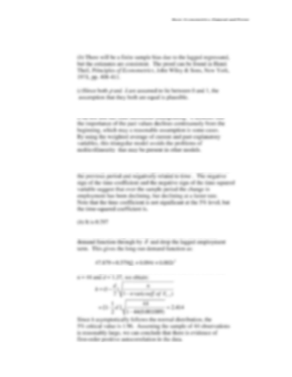
(a) On average, over the sample period, the change in employment
is positively related to output, negatively related to employment in
(c)To obtain the long-run demand curve, divide the short-run
(d) The appropriate test statistic here is the Durbin h. Given that
194
(
b
) The short-run price elasticity is –0.218, and the long-run price
17.16
The lagged term represents the combined influence of all the lagged
17.17
The degree of the polynomial should be at least one more than the
number of turning points in the observed time series plotted over
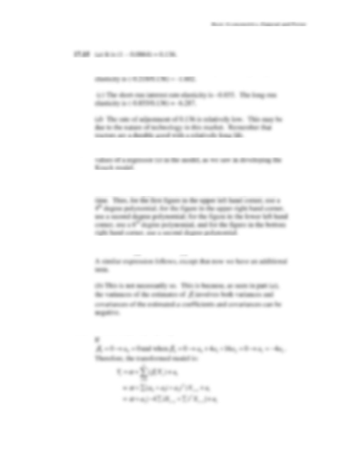
17.18
(
a
)
2
2
ˆ
ˆ ˆ ˆ
var( ) var( ) 2 cov( , )
p
j j p
i j j p
i a i a a
β
+
= +
∑ ∑
17.19
Given that
2
0 1 2
i
a a i a i
β
= + +
17.20
0
k
t i t i t
i
Y X u
α β
−
=
= + +
∑
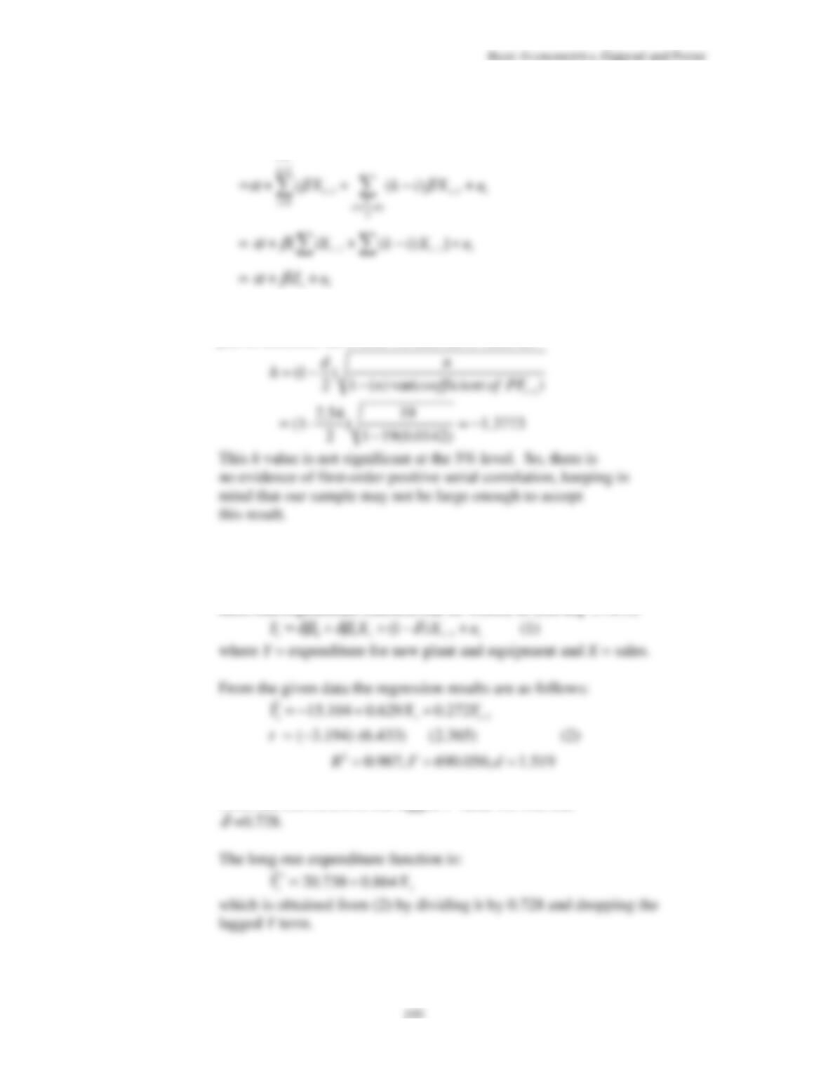
17.21
Here
n
= 19 and
d
= 2.54. Although the sample is not very large,
just to illustrate the
h
test, we find the
h
value as:
Empirical Exercises
17.22
Using the stock adjustment, or partial adjustment model (PAM), the
short-run expenditure function can be written as (see Eq. 17.6.5):
From the coefficient of the lagged
Y
value we find that
Basic Econometrics, Gujarati and Porter
196
We have to use the
h
statistic to find out if there is serial correlation
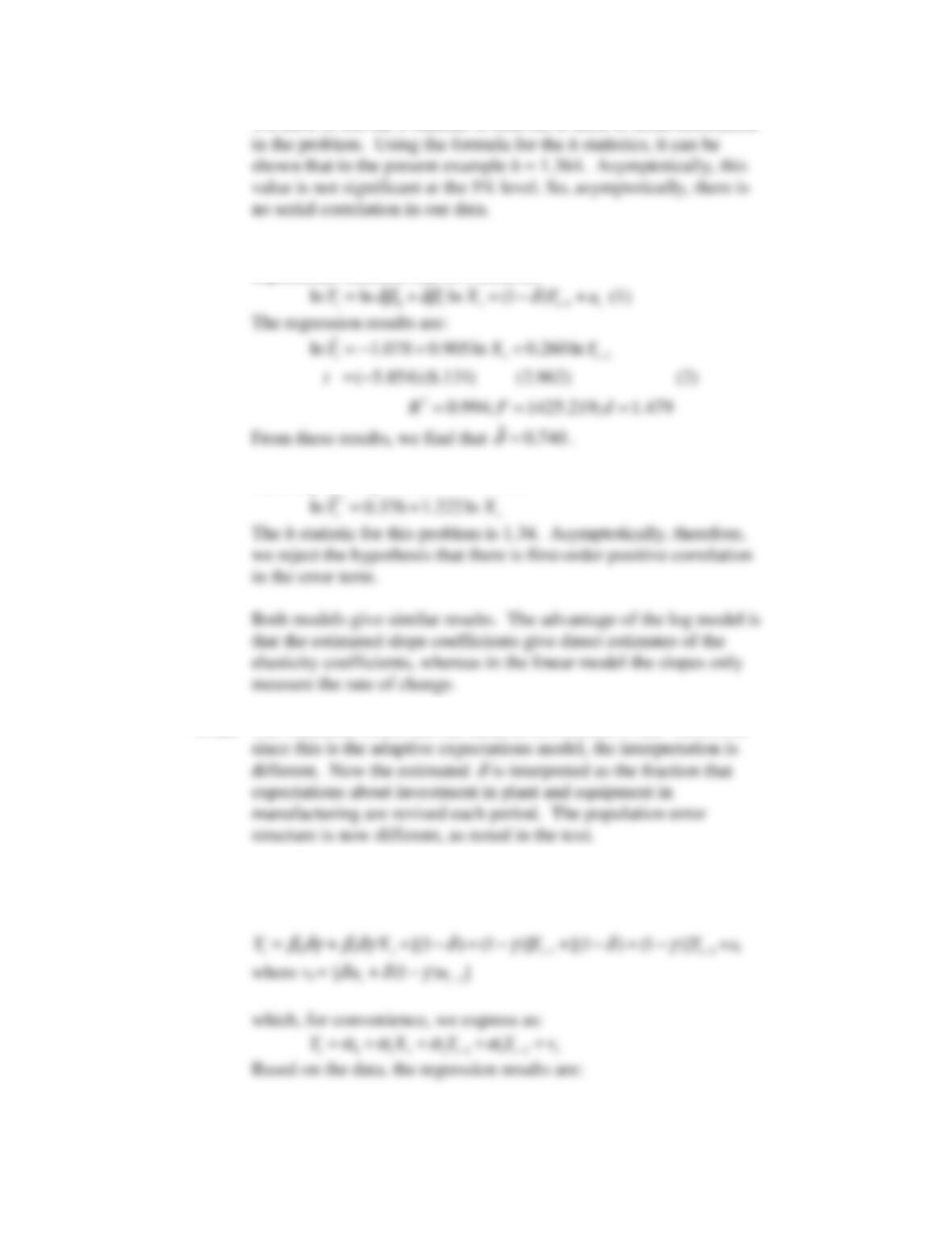
17.23
Using the same notation as in Exercise 17.22, the short-run
expenditure function can be written as:
The long-run expenditure function is:
17.24
The statistical results are the same as in Problem 17.22. However,
17.25
Here we use the combination of adaptive expectations and PAM.
The estimating equation is:
Basic Econometrics, Gujarati and Porter
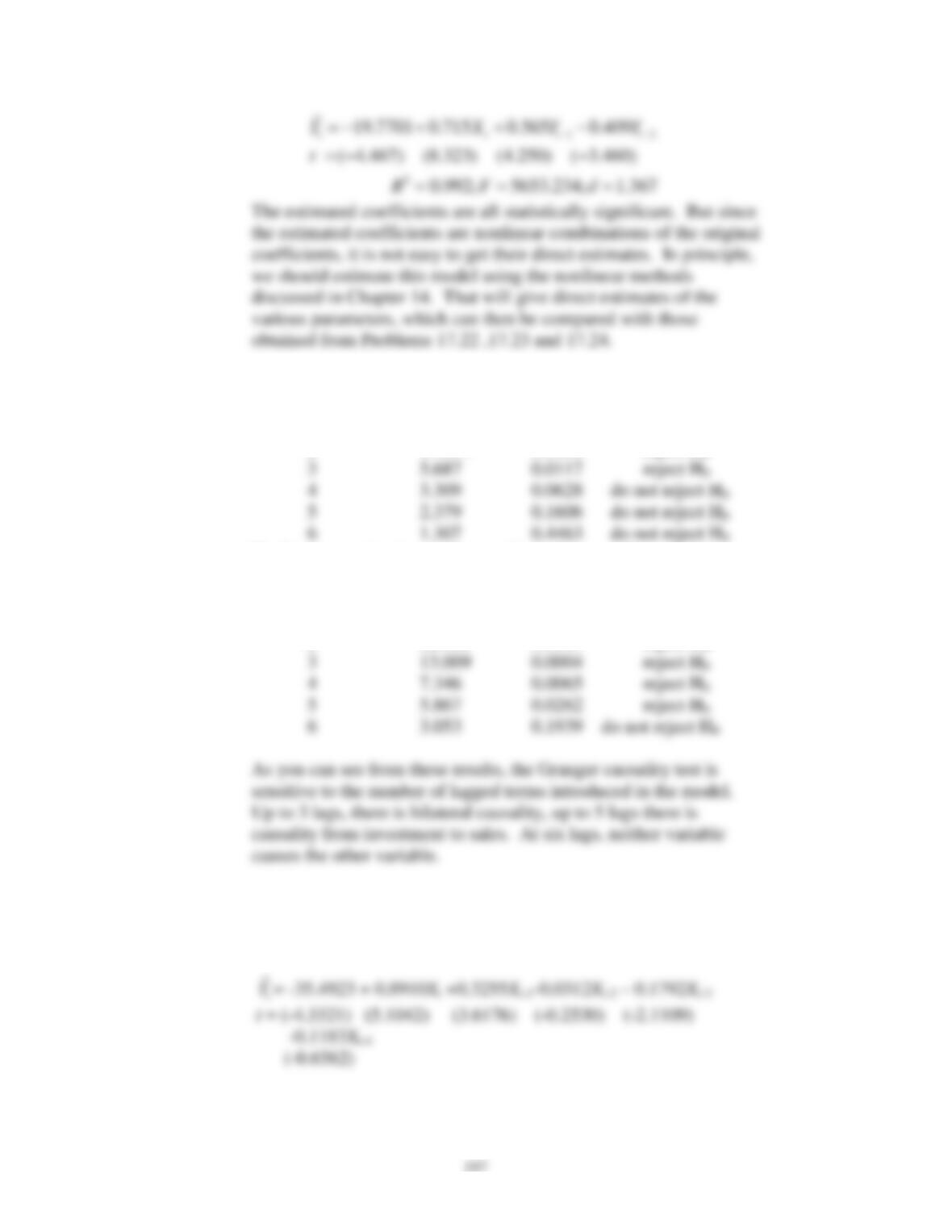
17.26
Null hypothesis H
0
: sales do not
Granger cause
investment in plant
and equipment. The results of the Granger test are as follows:
Number of lags F statistic p value Conclusion
2 17.394 0.0001 reject H
0
H
0
: Investment in plant and expenditure does not
Granger cause
sales:
Number of lags F statistic p value Conclusion
2 22.865 0.0001 reject H
0
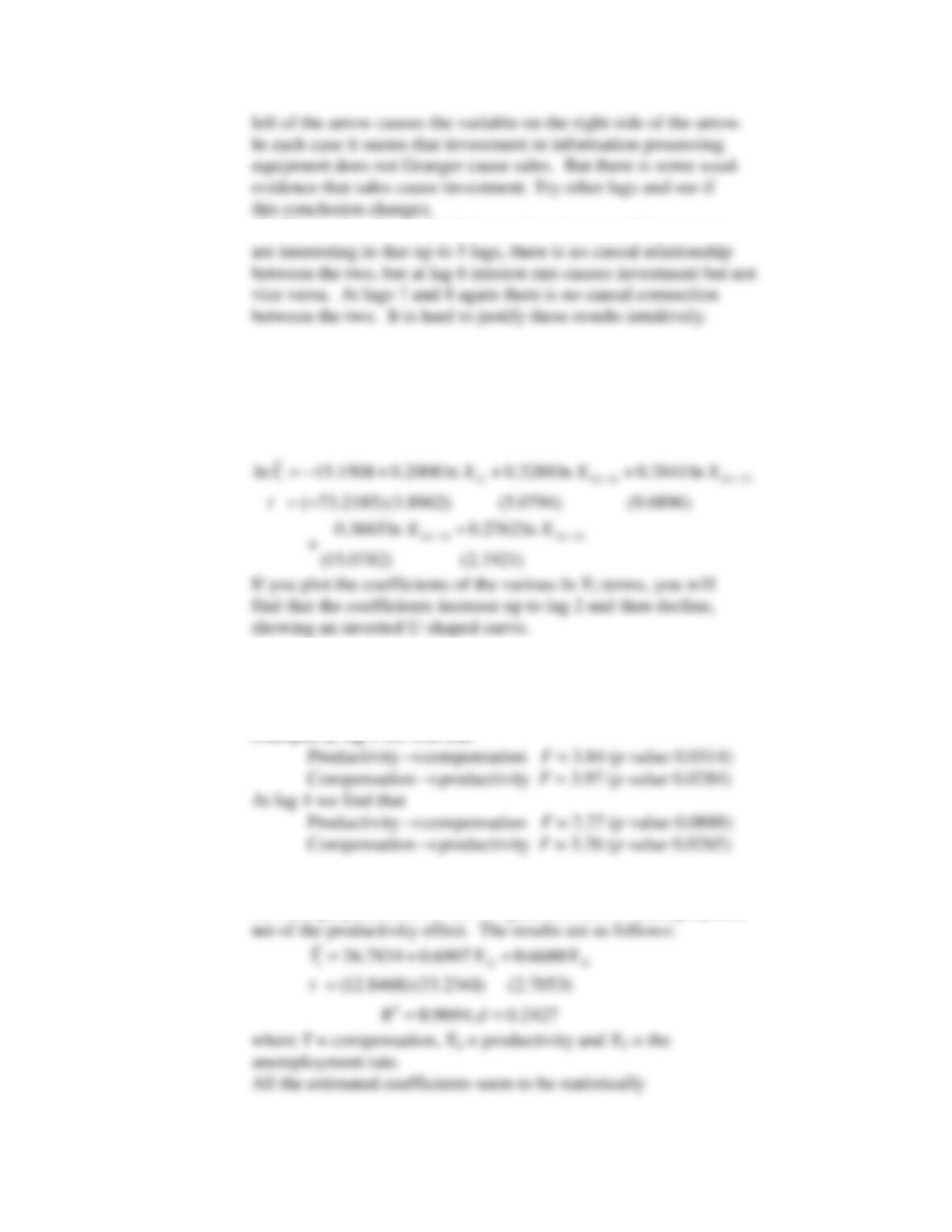
17.27
One illustrative model fitted here is a second degree polynomial
model with 4 lags. Using the format of Eq. (17.13.15) and letting
Y
represent investment and
X
sales, the regression results are:
The reader is urged to try other combinations of lags and the degree
Basic Econometrics, Gujarati and Porter
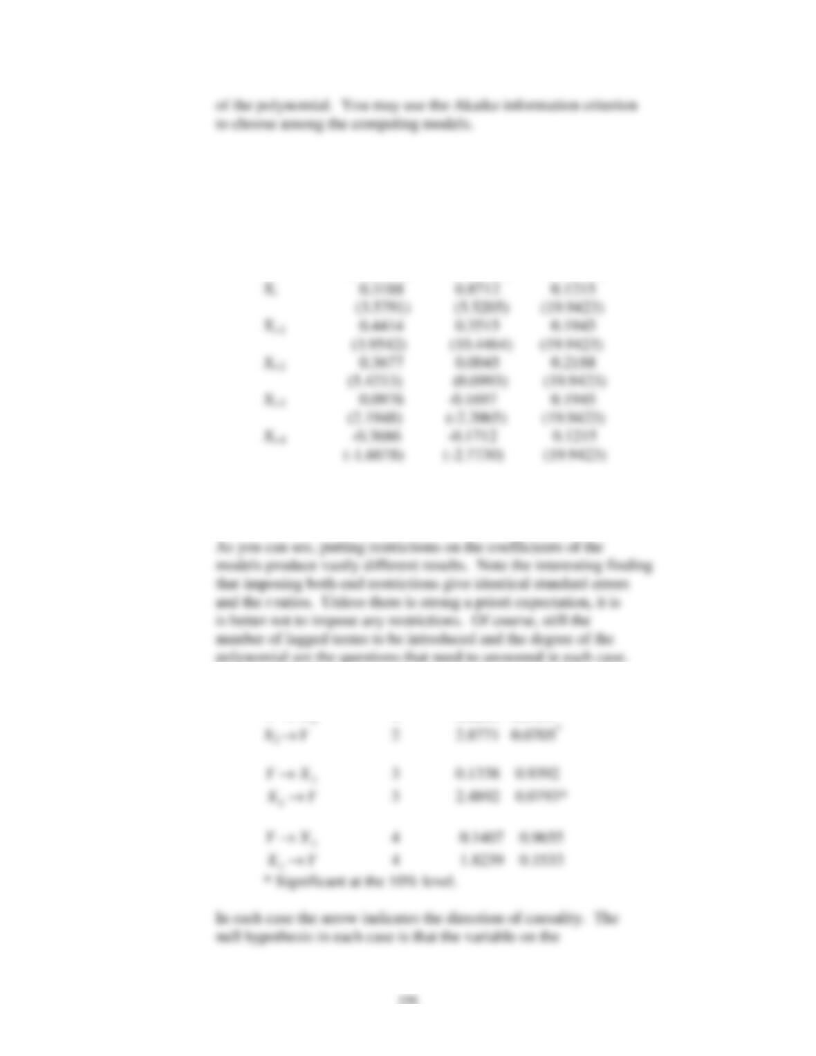
17.28
Using
EViews
, we obtained the following results.
Coefficient NER FER BER
Intercept -23.3844 -36.0936 -5.9303
( -2.3578) (-4.6740) (-0.8799)
Notes
: NER, FER, and BER denote near-end, far-end, and both-
end restrictions. Figures in the parentheses are the
t
ratios.
17.29
(
a
)
Direction of causality # of lags F Probability
Y X
→
2 0.0695 0.9329
Basic Econometrics, Gujarati and Porter
199
(
b
) The results of causality between investment and interest rate
(
c
)In the linear form there was no discernible distributed lag effect
of sales on investment. In the log-linear model with 4 lags and
second degree polynomial and imposing near end restriction, we get
the following results:
17.30 (a) & (b) Applying the Granger causality test, it can be shown that
up to 4 lags there is bilateral causality between the two variables, but
beyond 4 lags there is no unilateral or bilateral causality. For
(c)For example, we could regress compensation on productivity and
the unemployment rate to see the (partial) effect of unemployment
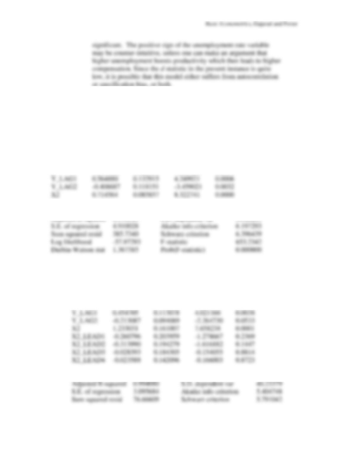
200
17.31 To perform the Sim‘s test, we ran Y (investment in plant
and equipment) on X (sales) with four lead terms of X and obtained
the following results for regression (1):
Dependent Variable: Y
Sample (adjusted): 3 22
Included observations: 20 after adjustments
Variable Coefficient Std. Error t-Statistic Prob.
C -19.77011 4.425609 -4.467207 0.0004
R-squared 0.991902 Mean dependent var 112.9975
Adjusted R-squared 0.990383 S.D. dependent var 50.06889
Dependent Variable: Y
Sample (adjusted): 3 18
Included observations: 16 after adjustments
Variable Coefficient Std. Error t-Statistic Prob.
C -0.871919 6.581770 -0.132475 0.8979
R-squared 0.996843 Mean dependent var 96.08000
Basic Econometrics, Gujarati and Porter
201
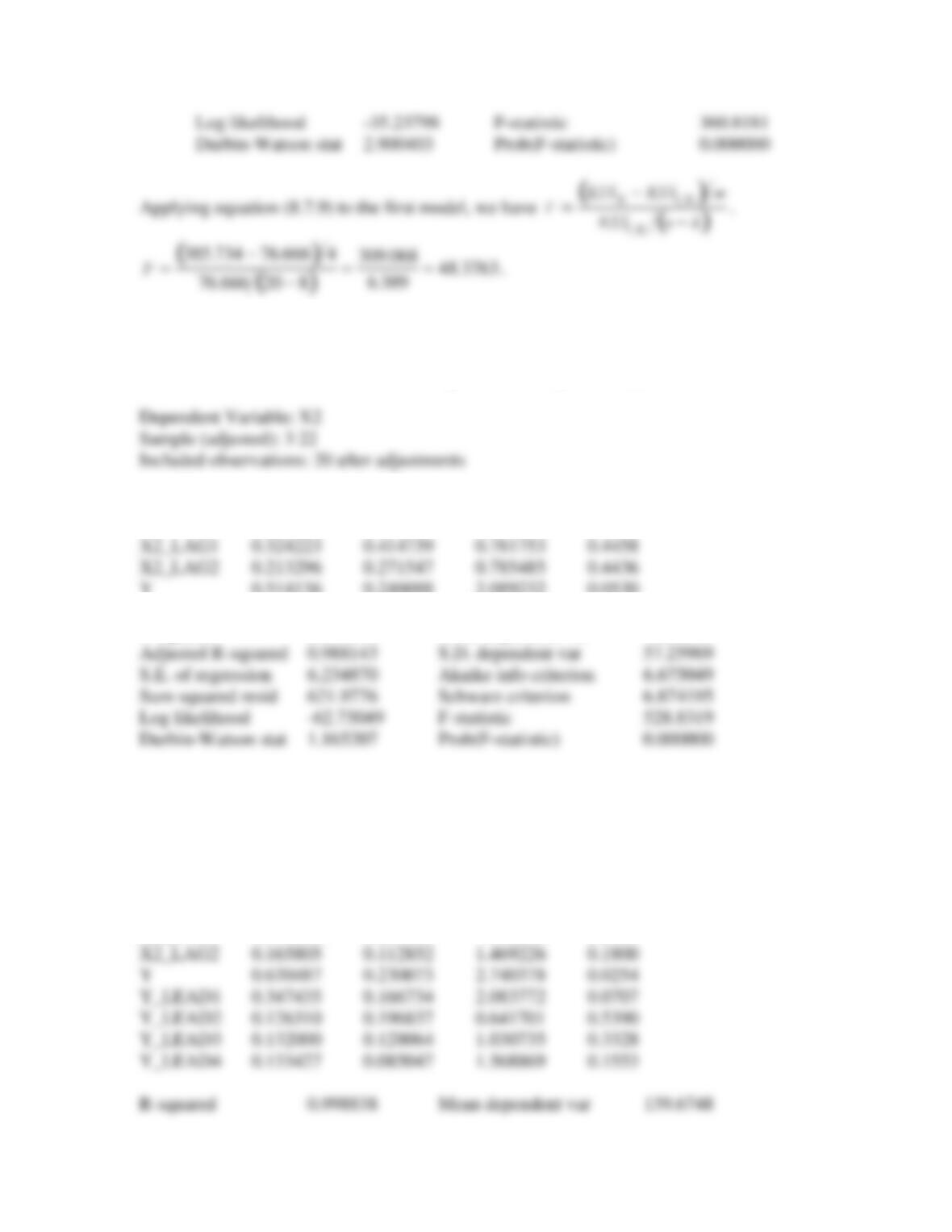
Now for model (2), we ran X (sales) on Y (investment in plant and equipment) four
lead terms of Y and obtained the following results for regression (2):
Variable Coefficient Std. Error t-Statistic Prob.
C 21.91458 6.145435 3.565994 0.0026
Y 0.514136 0.246088 2.089232 0.0530
R-squared 0.990016 Mean dependent var 158.2832
Dependent Variable: X2
Sample (adjusted): 3 18
Included observations: 16 after adjustments
Variable Coefficient Std. Error t-Statistic Prob.
C 14.26125 2.834342 5.031591 0.0010
X2_LAG1 -0.300083 0.269853 -1.112027 0.2984
Basic Econometrics, Gujarati and Porter
202
Adjusted R-squared 0.997822 S.D. dependent var 47.92886
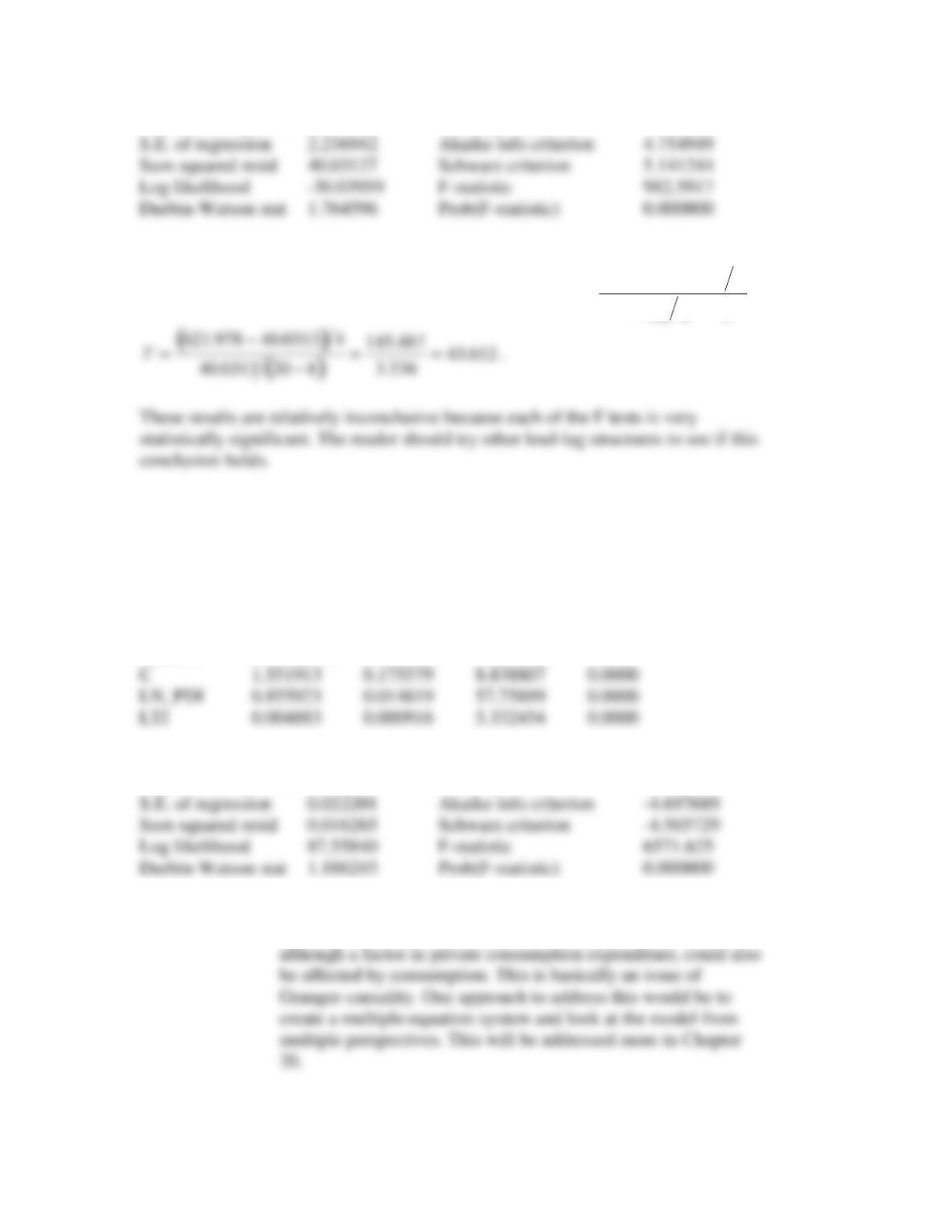
Applying equation (8.7.9) to the second model, we have
F=
RSS
R
−RSS
UR
(
)
m
RSS
UR
n−k
( )
.
17.32 (a) EViews results are:
Dependent Variable: LN_PC
Sample: 1960 1995
Included observations: 36
Variable Coefficient Std. Error t-Statistic Prob.
R-squared 0.997495 Mean dependent var 12.46542
Adjusted R-squared 0.997344 S.D. dependent var 0.430762
(b) An issue with estimation of the above model is that there could
be a “spurious” causality in effect. For example, the interest rate,
17.33 The model development here is left to the reader.