Economics Chapter 17 Homework This highlights an important result from the model: consumers can smooth

Unlock access to all the studying documents.

View Full Document

3. Calculate consumption each period based on the assumption that the country

wants to maintain the same level of consumption each period. Step 2 shows us

that PV(Q) = 2079 = PV(C). Therefore, we know that the present value of

4. Calculate the trade balance in each period. Now that we have pinned down output

and consumption, we can calculate the initial trade balance in the year of the

5. Calculate the country’s external wealth and the implied interest payments

paid/received on this debt to calculate net factor income from abroad (NFIA) in

6. Calculate the country’s current account in each period. Recall that the current

Generalizing Using the previous method, we can draw some general conclusions

regarding how consumption changes in response to changes in output in the open

The left–hand side represents the amount paid or received in interest on the amount

borrowed or lent. Solving for the change in consumption, we get

The value of r*/1 + r* must be between 0 and 1. That implies the open economy only

Smoothing Consumption When a Shock Is Permanent If a country faces a permanent

shock to output, then it will be forced to adjust its consumption regardless of whether it is

Summary: Save for a Rainy Day

The previous model shows how a country can save output when it experiences positive

S I D E B A R

Wars and the Current Account

In our example, we assumed no government spending (G). If we incorporate G into the

APPLICATION

Consumption Volatility and Financial Openness

Based on our model, countries with greater financial openness should be in a better

position to smooth consumption. In the data, we can measure this as the ratio of the

Why? In the real world, households are not identical and global capital markets are

not open to every individual or firm. In fact, some people and businesses do not even

participate in the domestic financial market. Thus, financial globalization doesn’t reach

consumers in poorer countries. Financial markets in emerging markets and developing

countries may not be fully developed, or may be limited in their access. Financial markets

in emerging market economies often function inefficiently, lacking transparency and

APPLICATION

Precautionary Saving, Reserves, and Sovereign Wealth Funds

If poorer countries are not able to rely on global financial markets, then what is their best

strategy to smooth consumption? One such approach is to rely on precautionary saving,

There are two general forms of precautionary saving: foreign reserves and sovereign

wealth funds. Foreign reserves are foreign assets owned by the central bank, often used

to maintain fixed exchange rates. Sovereign wealth funds are state-owned asset

management companies that invest government savings overseas in safe assets, such as

H E A D L I N E S

Copper–Bottomed Insurance

This article uses the case study of Chile as a copper exporter to discuss how the reliance

on export commodities can lead to output volatility, and how sovereign wealth funds can

help buffer against these shocks.

Background:

■ Chile’s government benefited from profits on its state-owned copper company

Key Statistics:

■ As of December 2014, there was $14.3 billion in the fund. This accounted for

5.4% of Chile’s GDP that year.

■ In 2014, the price of copper fell by 6% compared to 2013.

■ In current international dollars, per capita income in Chile was $23,367 (roughly

38% of Norway’s).

Lessons:

■ Commodity exports such as oil and copper are very volatile in price, and therefore

Discussion Questions:

■ Should Chile set aside these profits? Or should the government spend these profits

3 Gains from Efficient Investment

This section incorporates investment into the previous model, showing how financial

openness benefits the economy through not only consumption smoothing but also

increased investment opportunities.

The Basic Model

From the previous model, we can now assume that output is produced using capital,

which is accumulated through investment, so GNE = C + I. From the LRBC, we can

derive

As before, we will examine two cases:

■ Closed economy: TB = 0 in all periods, so the LRBC is automatically satisfied.

Efficient Investment: A Numerical Example and Generalization

We will consider the previous case, with shocks. Instead of a negative shock to output,

here, we consider a new investment opportunity in year 0. Assume the investment

opportunity requires 16 units of output today and will increase output by 5 units in every

subsequent period.

Before the shock, the present value of output is 2,100 and investment is equal to 0 in

each period. This is identical to the previous case with no shocks.

Now, consider what happens when the investment opportunity arises. To calculate the

implied changes in Q, C, I, TB, NFIA, and external wealth over time, we take steps

similar to the ones outlined previously.

Steps to computing numerical values for Q, C, TB, NFIA, and W over time are as

follows:

1. Identify how much output is needed to finance the investment project. From the

2. Calculate the present value of output, assuming the investment project is

undertaken:

Because Q0 = 100 and output is equal to 105 thereafter,

3. Calculate consumption each period, based on the assumption that the country

wants to maintain the same level of consumption each period. From Step 2, we

know PV(Q) = 2,200 = PV(C) + PV(I ). Therefore, we know that the present value

of consumption is 2,184 (= 2,200 − 16), to be divided equally each period (e.g., to

keep consumption smooth), so C0 = C1 = C2 = C:

4. Calculate the trade balance in each period. Now that we have determined output,

investment, and consumption, we can calculate the initial trade balance in the year

5. Calculate the country’s external wealth and the implied interest payments paid or

received on this debt to calculate NFIA in each period. External wealth is equal to

6. Calculate the country’s current account in each period. Recall that the current

account is the sum of the trade balance, net factor income, and net unilateral

Generalizing The country’s objective is to maximize the present value of consumption.

There are investment projects that are not worthwhile because they do not increase output

enough to increase the present value of consumption. To determine which investment

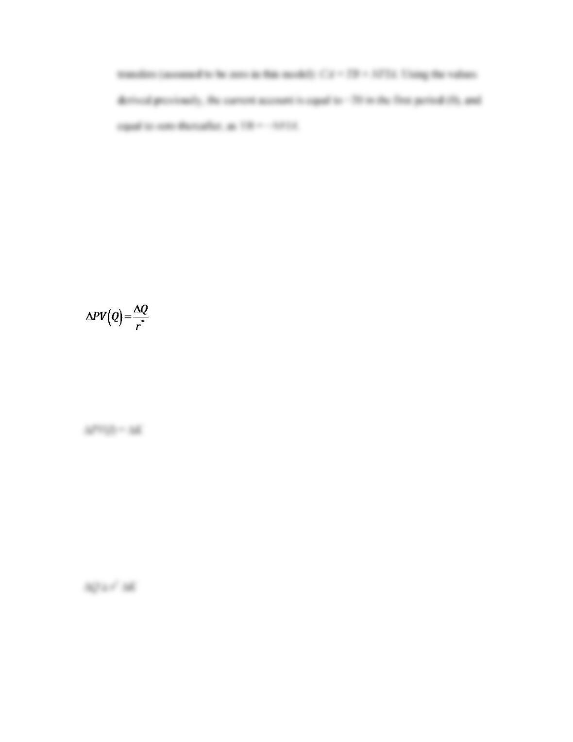
projects are worthy, note that the change in the present value of output is

The change in the present value of investment (equal to the change in capital stock, K) is

The investment project is worthwhile only if the present value of output increases (gains

from the project) more than the present value of investment (cost of the project financed

through borrowing):

The left-hand side shows the annual benefit of the project and the right-hand side is the

cost (interest payments on the debt accumulated). Rearranging the expression gives us

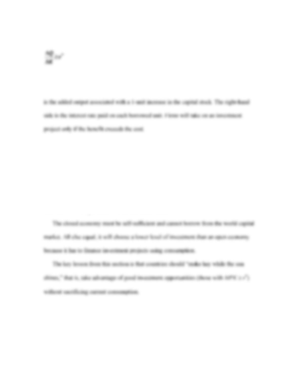
The left-hand side of this expression is the marginal product of capital (MPK), which

Summary: Make Hay While the Sun Shines

In an open economy, a country is able to separate its consumption and investment

decisions. Firms and households can borrow or save through the world capital market. To

choose an efficient level of investment, the country should undertake investment projects

until the MPK is equal to the world real interest rate.

APPLICATION

Delinking Saving from Investment

A massive oil reserve was discovered in the North Sea in the 1960s, but it was very costly

to extract this oil at the time. The world price of oil was low until the oil price shocks in

the 1970s. These shocks turned out to be largely permanent, leading to a permanent

increase in the price of oil that then made the extraction of North Sea oil profitable.

Is this delinking of saving and investment a general result? Feldstein and Horioka

estimated a ratio

—the fraction of each additional dollar saved that tended to be invested

in the same country (∆I =

∆S). According to our model for financially open economies,

Can Poor Countries Gain from Financial Globalization?

The previous model shows us that countries with MPK > r* should borrow from abroad to

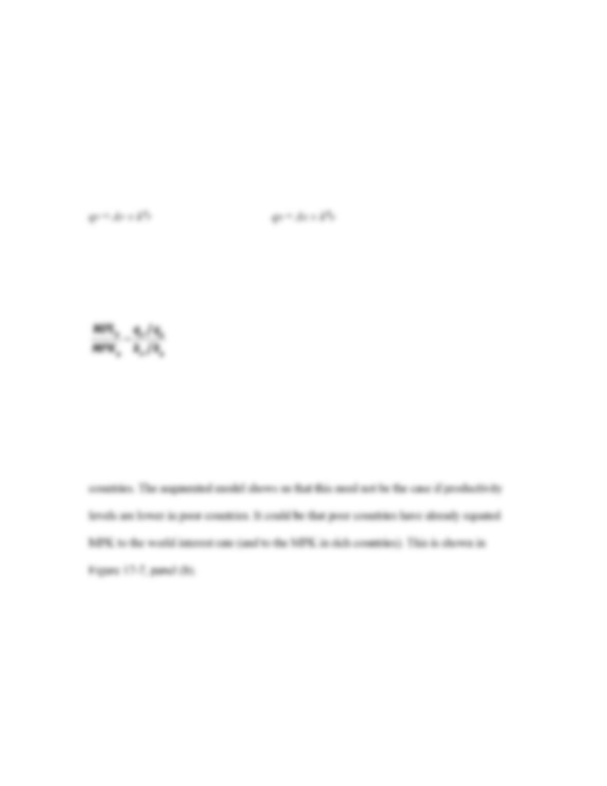
Production Function Approach A production function describes how a country’s output

depends on its inputs. In per worker terms, the production function describes the

relationship between capital per worker (k = K/L) and productivity (q = Q/L). The simple

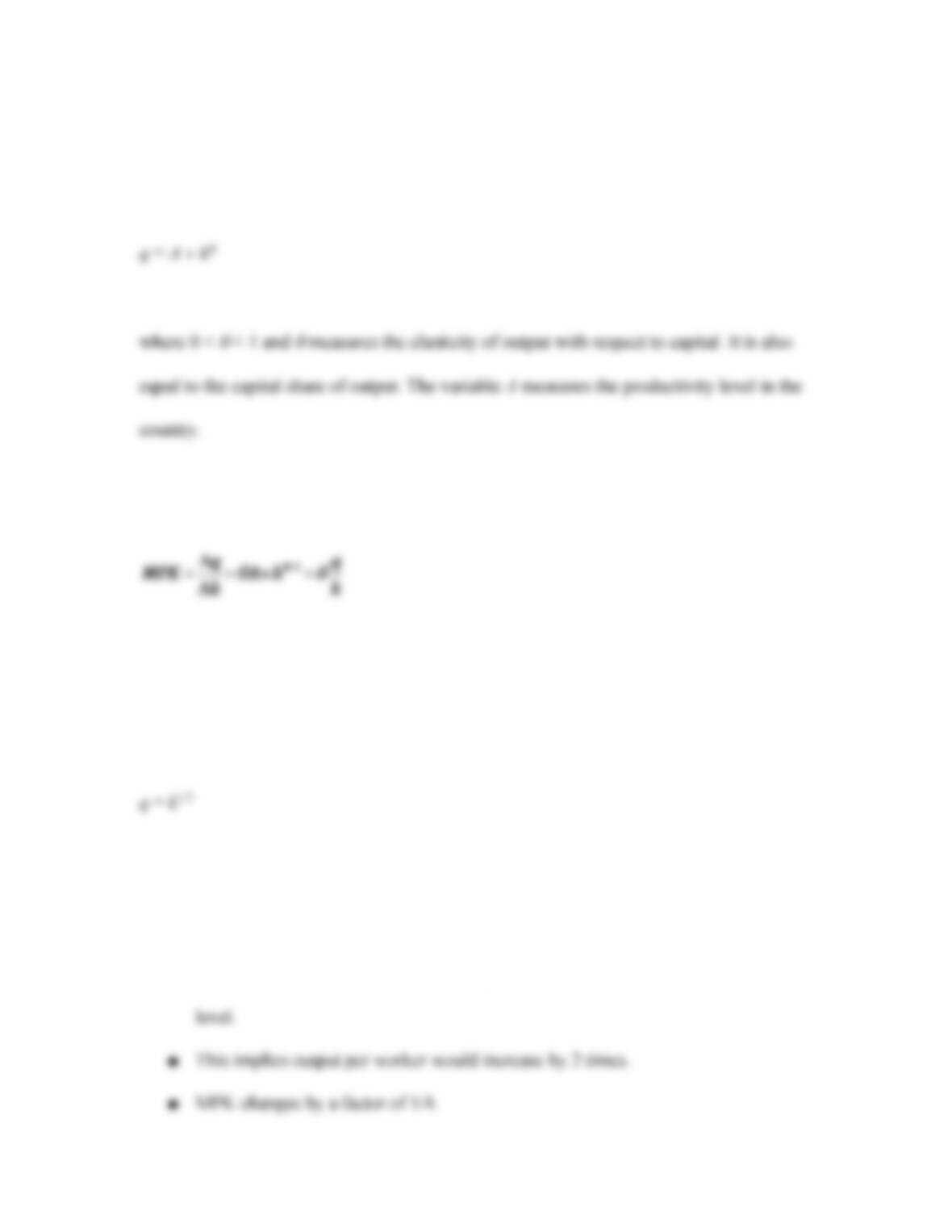
production function used here is

To determine the efficient level of investment, we need to know the MPK:

where MPK is the slope of the production function. The textbook plots the production

function for the case where A = 1 and = 1/3:

A Benchmark Model: Countries Have Identical Productivity Levels This model

assumes that all countries have the same production function.

■ Suppose a country considers increasing its capital per work by 8 times the current

Now, we consider two different countries.

■ Suppose that a poor country has half the level of output per worker enjoyed in the

rich country.

■ The poor country has an MPK 4 times that of the rich country.

The general result is that the poorer the country, the lower its capital per worker and

therefore the higher its MPK. This relationship is illustrated on Figure 17-7, panel (a).

The Lucas Paradox: Why Doesn’t Capital Flow from Rich to Poor Countries?

The implication from the previous model is clear: capital should flow from rich to poor

countries, and poor countries should implement government policies to attract capital

inflow.

An Augmented Model: Countries Have Different Productivity Levels The augmented

model allows for different countries to have different productivity levels—different

values for A. Let the subscript P denote a poor country and the subscript R denote a rich

country:

The ratio of the MPK in each country is

We can use this expression to understand why the naïve model overlooks a key source of

differences in output per worker—differences in the production function, A. The

benchmark model predicts the MPK in poor countries is much higher than that in rich

APPLICATION

A Versus k

Table 17-5 compares the ratio of output per worker and capital per worker in selected

countries to those in the United States. These ratios can be used to calculate the implied

difference in the productivity levels in poor countries relative to the United States. From

the table, we observe that the implied gains from the benchmark model are much larger

than those implied by the augmented model.

More Bad News? There are other assumptions in the model that we could relax to study

a richer set of explanations for why capital does not flow from rich to poor countries:

■ The model makes no allowance for risk premiums. The existence of a risk

■ Risk premiums may be large enough to cause capital to flow “uphill” from poor

less attractive.

■ The model assumes that investment goods can be acquired at the same relative

■ The model assumes the contribution of capital to production is equal across

■ The model suggests that foreign aid may do no better than foreign investors in

promoting growth. Investments from foreign aid face the same challenges faced

S I D E B A R

What Does the World Bank Do?

The World Bank (http://www.worldbank.org) was established in 1944 as part of the

Bretton Woods Agreement. (Its “twin,” the International Monetary Fund, was set up at

H E A D L I N E S

A Brief History of Foreign Aid

This article considers the role of foreign aid in economic growth.

Background:

■ In 1985, Live Aid concerts were performed to raise funds to fight poverty in

Africa.

and received aid.

Lessons:

■ During the Cold War, much foreign aid was offered more for geopolitical

purposes than to promote economic growth, so historical analysis of the effects of

aid may be misleading.

Discussion Questions:

■ What criteria would you establish in offering aid to poor countries?

4 Gains from Diversification of Risk

In the previous section, we observed that in practice, countries may not have access to the

world capital market. Are there other ways to cope with shocks to output? Yes, through

Diversification: A Numerical Example and Generalization

In this section, we assume there are two countries with no borrowing/lending. The two

countries are identical, except that their outputs move in opposite directions. We will

Home Portfolios Assume the countries are closed. In this case, each country owns 100%

World Portfolios Table 17-6, panels (b) and (c), shows outcomes when each country