Unlock document.
This document is partially blurred.
Unlock all pages and 1 million more documents.
Get Access

Questions for Review
1. First, Keynes conjectured that the marginal propensity to consume—the amount con-
sumed out of an additional dollar of income—is between zero and one. This means that
if an individual’s income increases by a dollar, both consumption and saving increase.
Second, Keynes conjectured that the ratio of consumption to income—called the
2. The evidence that was consistent with Keynes’s conjectures came from studies of house-
hold data and short time-series. There were two observations from household data.
First, households with higher income consumed more and saved more, implying that
the marginal propensity to consume is between zero and one. Second, higher-income
households saved a larger fraction of their income than lower-income households,
3. Both the life-cycle and permanent-income hypotheses emphasize that an individual’s
time horizon is longer than a single year. Thus, consumption is not simply a function of
current income.
The life-cycle hypothesis stresses that income varies over a person’s life; saving
allows consumers to move income from those times in life when income is high to those
CHAPTER 17 Consumption
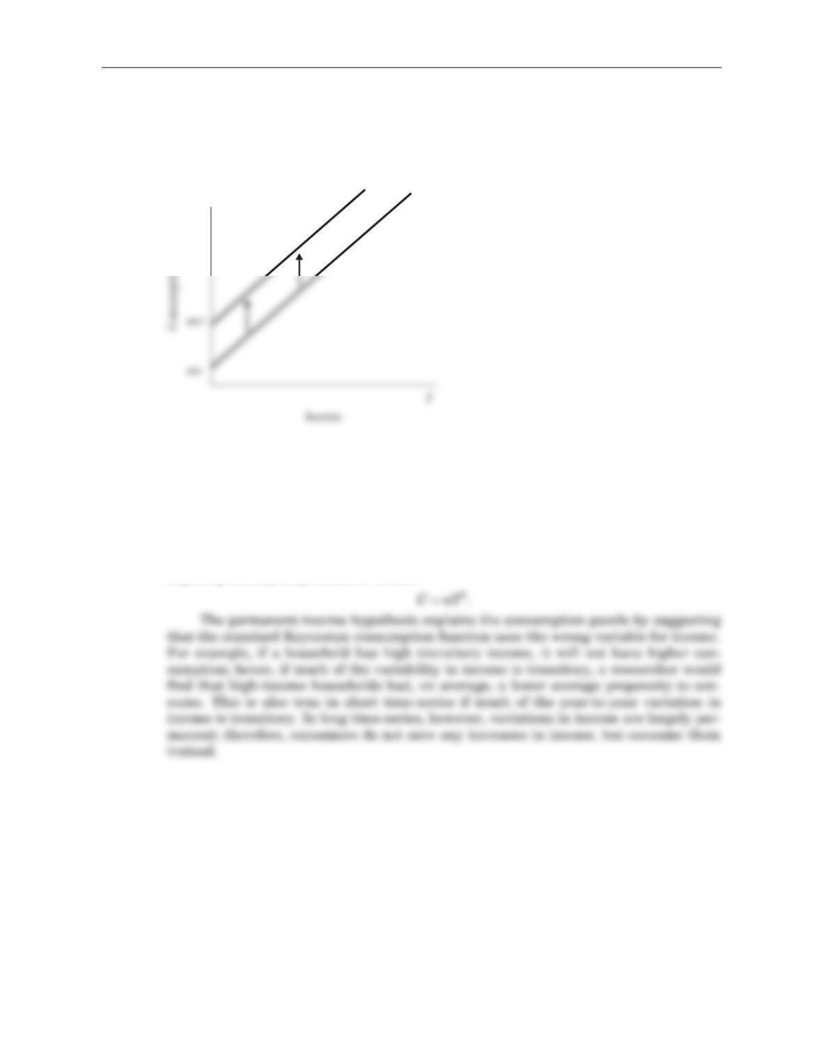
In the short run, with wealth fixed, we get a “conventional” Keynesian consumption
function. In the long run, wealth increases, so the short-run consumption function
shifts upward, as shown in Figure 17–1.
The permanent-income hypothesis also implies that people try to smooth con-
sumption, though its emphasis is slightly different. Rather than focusing on the pat-
tern of income over a lifetime, the permanent-income hypothesis emphasizes that peo-
ple experience random and temporary changes in their income from year to year. The
permanent-income hypothesis views current income as the sum of permanent income
Ypand transitory income Yt. Milton Friedman hypothesized that consumption should
depend primarily on permanent income:
176 Answers to Textbook Questions and Problems
C
Figure 17–1
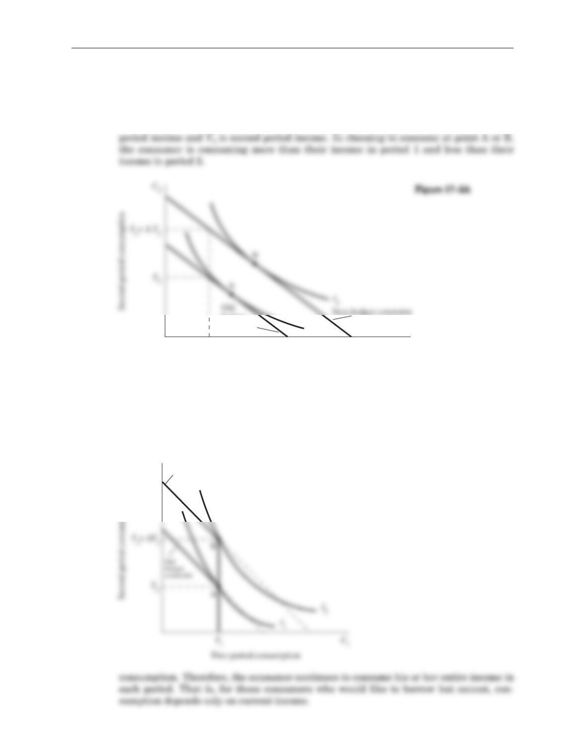
4. Fisher’s model of consumption looks at how a consumer who lives two periods will
make consumption choices in order to be as well off as possible. Figure 17–2(A) shows
the effect of an increase in second-period income if the consumer does not face a binding
borrowing constraint. The budget constraint shifts outward, and the consumer increas-
es consumption in both the first and the second period. In Figure 17-2(A), Y1is the first
Figure 17–2(B) shows what happens if there is a binding borrowing constraint.
The consumer would like to borrow to increase first-period consumption but cannot. If
income increases in the second period, the consumer is unable to increase first-period
Chapter 17 Consumption 177
I1
C1
Y1
First-period consumption
budget
constraint
New
budget
constraint
C2
Figure 17–2B

5. The permanent-income hypothesis implies that consumers try to smooth consumption
over time, so that current consumption is based on current expectations about lifetime
income. It follows that changes in consumption reflect “surprises” about lifetime
income. If consumers have rational expectations, then these surprises are unpre-
dictable. Hence, consumption changes are also unpredictable.
Problems and Applications
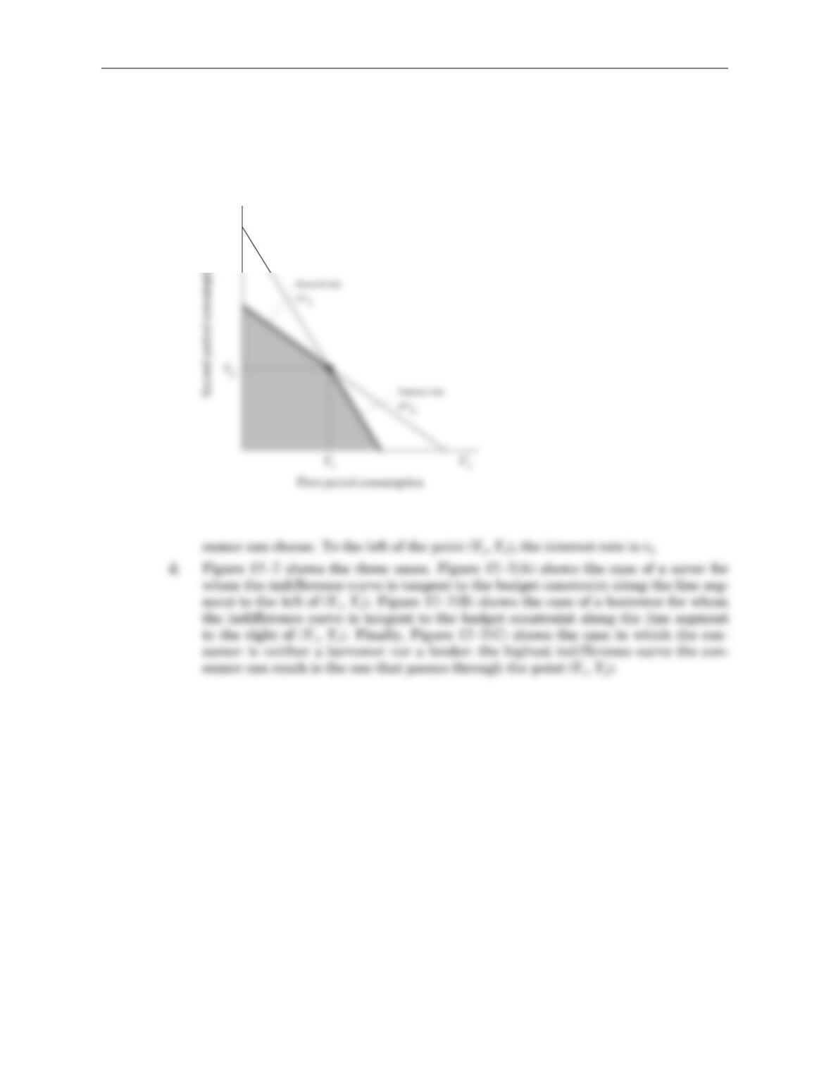
1. Figure 17–3 shows the effect of an increase in the interest rate on a consumer who bor-
rows in the first period. The increase in the real interest rate causes the budget line to
rotate around the point (Y1, Y2), becoming steeper.
We can break the effect on consumption from this change into an income and sub-
stitution effect. The income effect is the change in consumption that results from the
movement to a different indifference curve. Because the consumer is a borrower, the
increase in the interest rate makes the consumer worse off—that is, he or she cannot
achieve as high an indifference curve. If consumption in each period is a normal good,
this tends to reduce both C1and C2.
New budget
constraint
C2
Figure 17–3
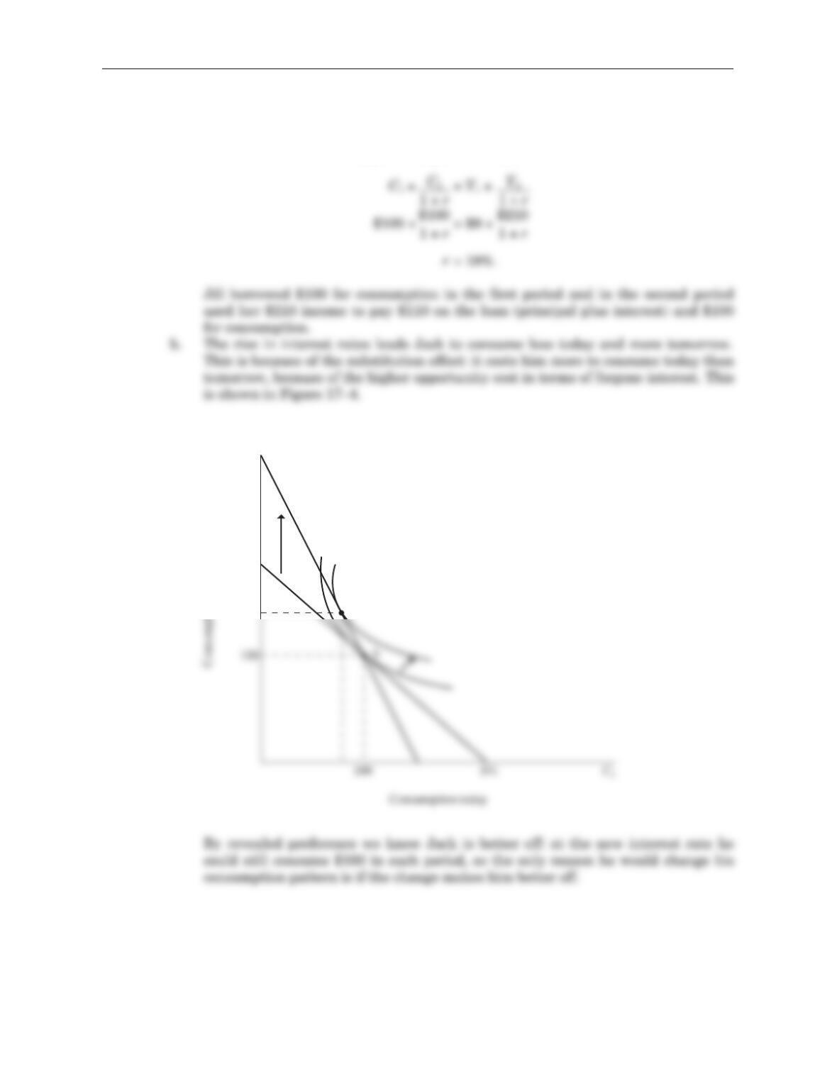
effect is stronger. In Figure 17–3, we show the case in which the substitution effect is
stronger than the income effect, so that C2increases.
2. a. We can use Jill’s intertemporal budget constraint to solve for the interest rate:
Chapter 17 Consumption 179
B
210
C2
Figure 17–4
180 Answers to Textbook Questions and Problems
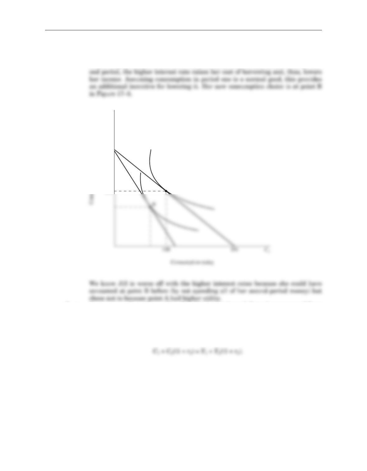
c. Jill consumes less today, while her consumption tomorrow can either rise or fall.
She faces both a substitution effect and income effect. Because consumption today
is more expensive, she substitutes out of it. Also, since all her income is in the sec-
3. a. A consumer who consumes less than his income in period one is a saver and faces
an interest rate rs. His budget constraint is
C1+ C2/(1 + rs) = Y1+ Y2/(1 + rs).
b. A consumer who consumes more than income in period one is a borrower and faces
an interest rate rb. The budget constraint is
A
100
210
C2
Figure 17–5
Chapter 17 Consumption 181
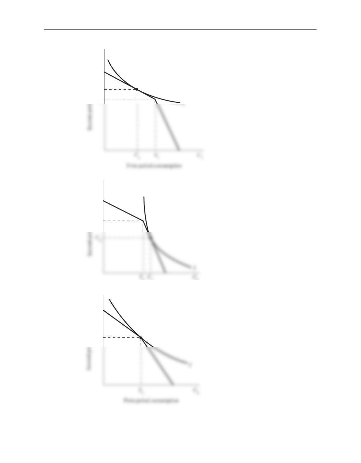
c. Figure 17–6 shows the two budget constraints; they intersect at the point (Y1, Y2),
where the consumer is neither a borrower nor a lender. The shaded area repre-
sents the combinations of first-period and second-period consumption that the con-
C2
Figure 17–6
182 Answers to Textbook Questions and Problems
C2
C2
Y2
Figure 17–7A
C2
Y2
Figure 17–7B
C2
Y2
Figure 17–7C
Chapter 17 Consumption 183
e. If the consumer is a saver, then consumption in the first period depends on [Y1+
Y2/(1 + rs)]—that is, income in both periods, Y1and Y2, and the interest rate rs. If
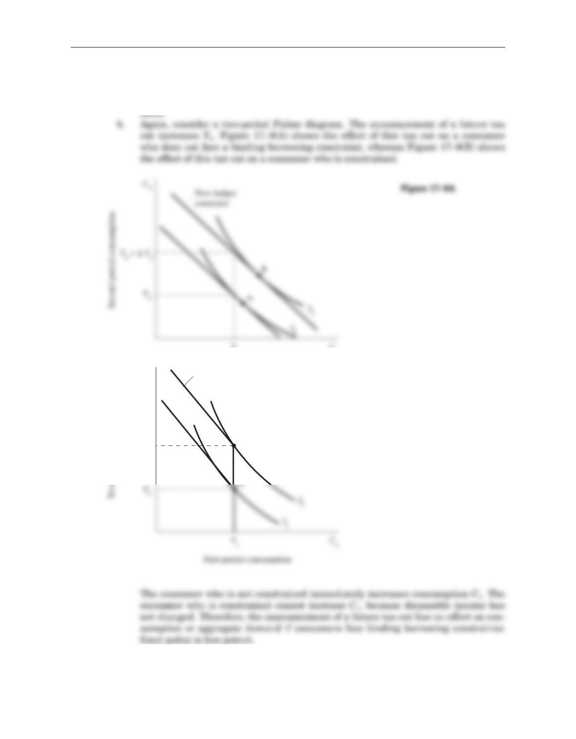
4. The potency of fiscal policy to influence aggregate demand depends on the effect on con-
sumption: if consumption changes a lot, then fiscal policy will have a large multiplier.
If consumption changes only a little, then fiscal policy will have a small multiplier.
That is, the fiscal-policy multipliers are higher if the marginal propensity to consume is
higher.
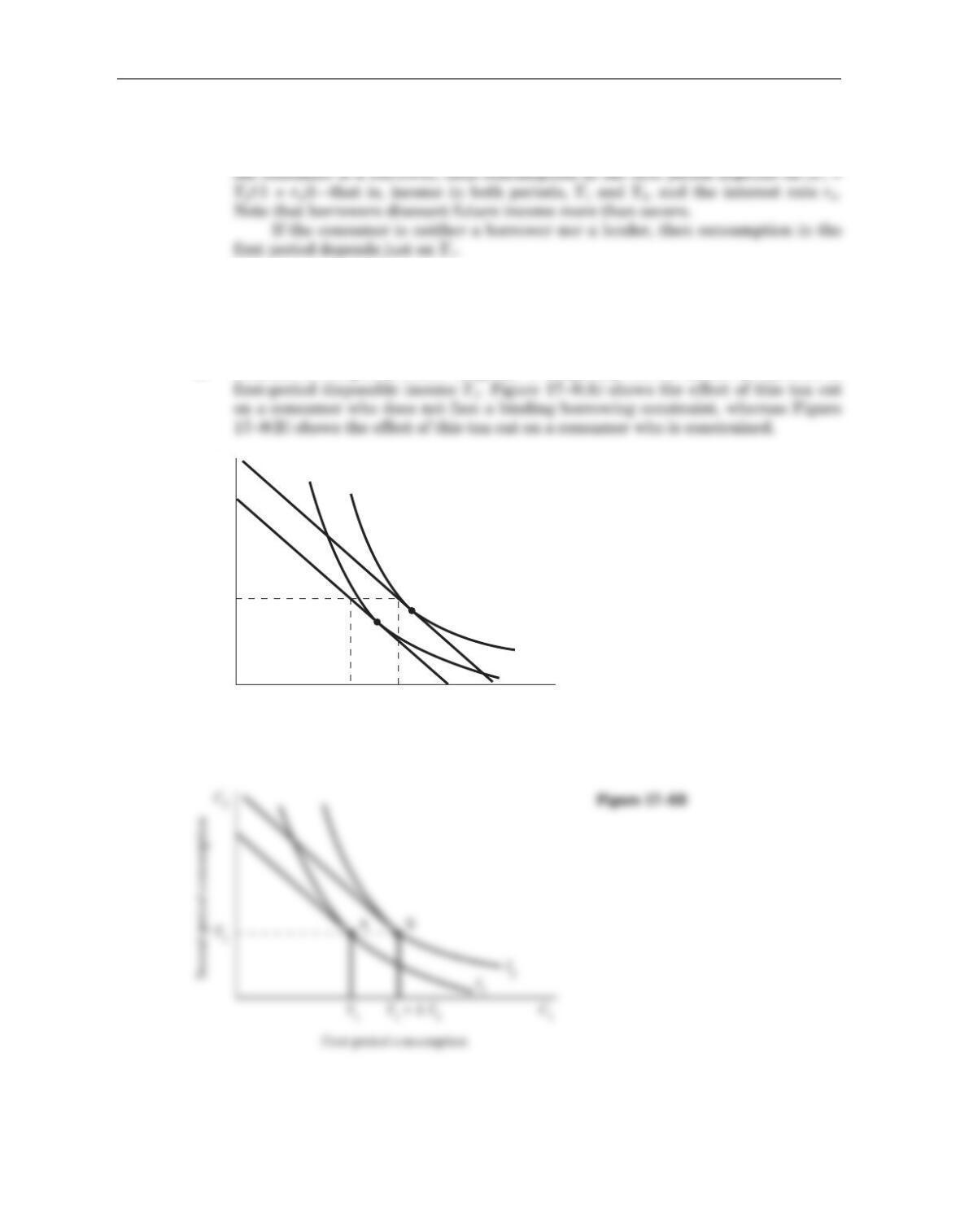
a. Consider a two-period Fisher diagram. A temporary tax cut means an increase in
The consumer with the constraint would have liked to get a loan to increase C1,
but could not. The temporary tax cut increases disposable income: as shown in the
figure, the consumer’s consumption rises by the full amount that taxes fall. The
consumer who is constrained thus increases first-period consumption C1by more
AB
C2
Y2
Y1 + Δ Y1
Y1
First-period consumption
I1
C1
I2
Figure 17–8A
184 Answers to Textbook Questions and Problems
than the consumer who is not constrained—that is, the marginal propensity to
consume is higher for a consumer who faces a borrowing constraint. Therefore, fis-
cal policy is more potent with binding borrowing constraints than it is without
5. In this question, we look at how income growth affects the pattern of consumption and
wealth accumulation over a person’s lifetime. For simplicity, we assume that the inter-
est rate is zero and that the consumer wants as smooth a consumption path as possible.
a. Figure 17–10 shows the case in which the consumer can borrow. Income increases
during the consumer’s lifetime until retirement, when it falls to zero.
B
C1
Y1
C2
Y2 + Δ Y2
New budget
constraint
Figure 17–9B
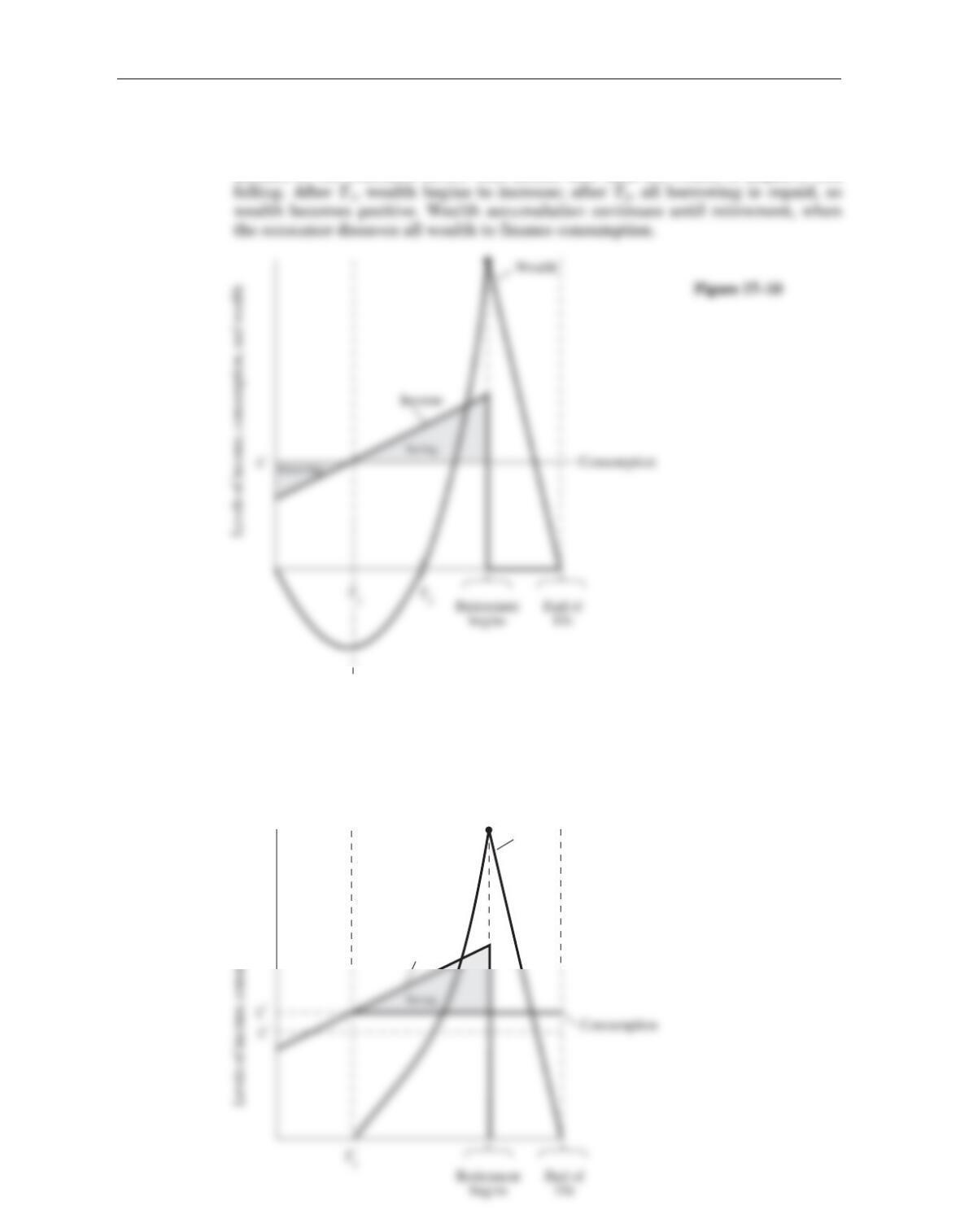
Desired consumption is level over the lifetime. Until year T1, consumption is
greater than income, so the consumer borrows. After T1, consumption is less than
income, so the consumer saves. This means that until T1, wealth is negative and
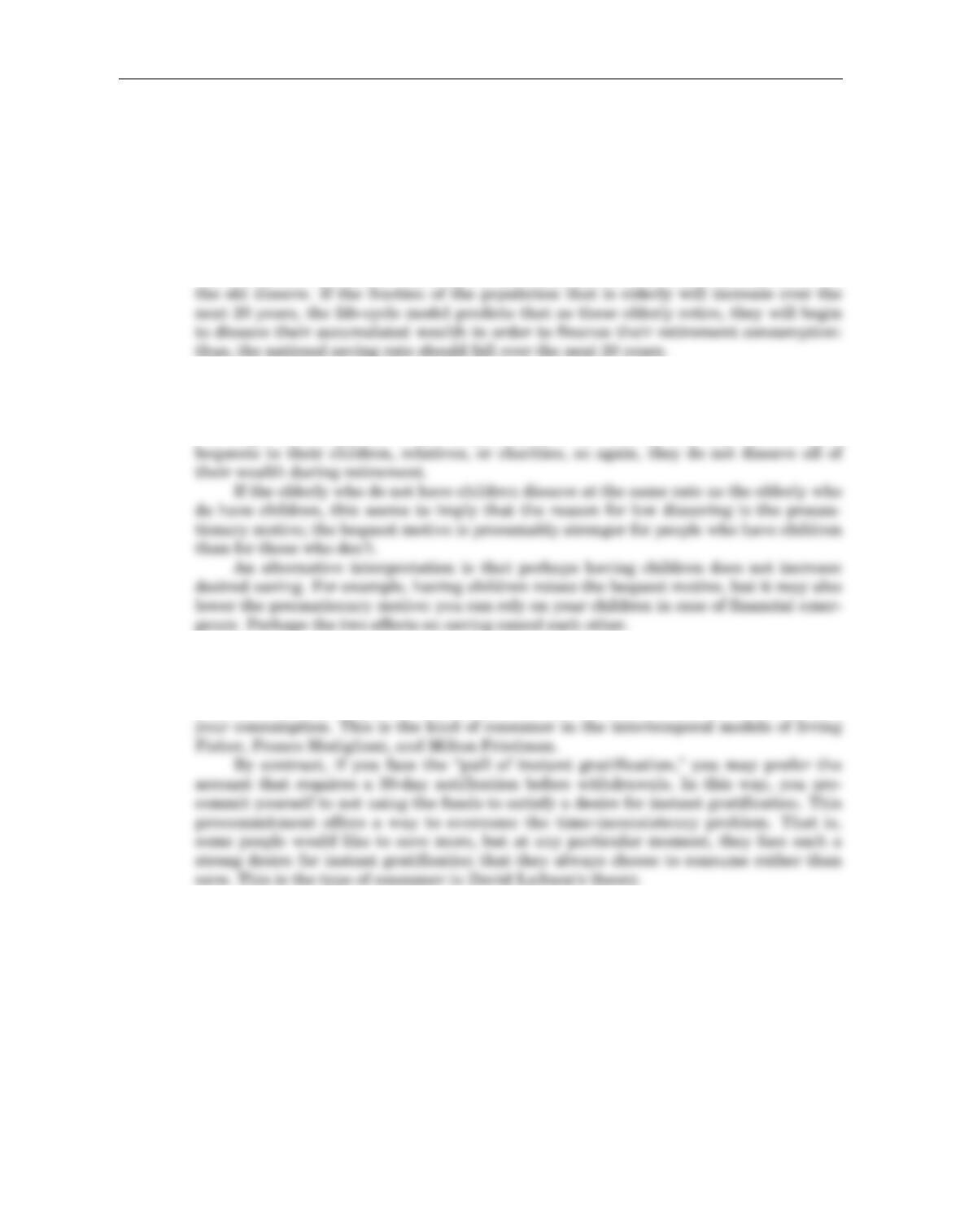
b. Figure 17–11 shows the case in which a borrowing constraint prevents the consumer
from having negative wealth. Before T1′, the consumer would like to be borrowing,
as in part (a), but cannot. Therefore, income is consumed and is neither saved nor
borrowed. After T1′, the consumer begins to save for retirement, and lifetime con-
sumption remains constant at C′. In Figure 17-11 the consumption path has con-
sumption rising up to time T1′, and then consumption remains constant at C′.
Chapter 17 Consumption 185
Wealth
Income
Figure 17–11
186 Answers to Textbook Questions and Problems
Note that C′is greater than C, and T1′is greater than T1, as shown. This is
because in part (b), the consumer has lower consumption in the first part of life, so
there are more resources left when there is no constraint—consumption will be
higher. The case where people are borrowing constrained in their early working
years is more realistic since it is difficult, if not impossible, to borrow against
expected future income.
6. The life-cycle model predicts that an important source of saving is that people save
while they work to finance consumption after they retire. That is, the young save, and
7. In this chapter, we discussed two explanations for why the elderly do not dissave as
rapidly as the life-cycle model predicts. First, because of the possibility of unpredictable
and costly events, they may keep some precautionary saving as a buffer in case they
live longer than expected or have large medical bills. Second, they may want to leave
8. If you are a fully rational and time-consistent consumer, you would certainly prefer the
saving account that lets you take the money out on demand. After all, you get the same
return on that account, but in unexpected circumstances (e.g., if you suffer an unex-
pected, temporary decline in income), you can use the funds in the account to finance


