Unlock document.
This document is partially blurred.
Unlock all pages and 1 million more documents.
Get Access
CHAPTER 17
The Theory of Investment
Notes to the Instructor
Chapter Summary
Chapter 17 examines the determinants of investment in greater detail. It examines three different
components of investment in turn: business fixed investment, residential investment, and
inventory investment. The first section explains the neoclassical theory of the cost of capital,
Tobin’s q, and financing constraints; the second section provides a simple model of the housing
market; and the third discusses the motives for holding inventories.
Comments
One potential problem in this chapter involves explaining why it presents three different theories
of investment. A way to circumvent or at least mitigate this is to stress that all three theories
Use of the Dismal Scientist Web Site
Go to the Dismal Scientist Web site and download quarterly data on the major components of
investment expenditures (business fixed, residential, and inventory) in the United States over the
past ten years. Assess the effect of the recession of 2001 and the recession of 2008–2009 on
investment spending. Did it decline during these recessions? Did certain components decline but
not others? The 2008–2009 recession has been accompanied by a substantial decline in the stock
market and a severe contraction in the availability of credit. What components of investment
would you expect this to most affect? Do the data confirm your expectation?
Chapter Supplements
This chapter includes the following supplements:
17-2 Asset Pricing I: Why Do We Care?
17-3 Asset Pricing II: Stock Prices and Efficient Markets
17-5 Asset Pricing IV: Bubbles, Excess Volatility, and Fads
17-7 Financing Constraints in Japanese Firms
17-9 The Tax Treatment of Housing

17-10 The Importance of Inventories
17-12 Production Smoothing and Coordination Failure
17-14 Additional Readings
Lecture Notes | 397
Lecture Notes
Introduction
17-1 Business Fixed Investment
We explain business fixed investment using the neoclassical model of investment. The simplest
explanation of this approach makes use of a convenient fiction. We suppose that the firms in the
economy can be divided into two types: production firms, which rent capital and labor to
produce goods, and rental firms, which own capital and rent it out to production firms. Although
most firms own their capital rather than renting it, this trick simplifies our analysis without being
The Rental Price of Capital
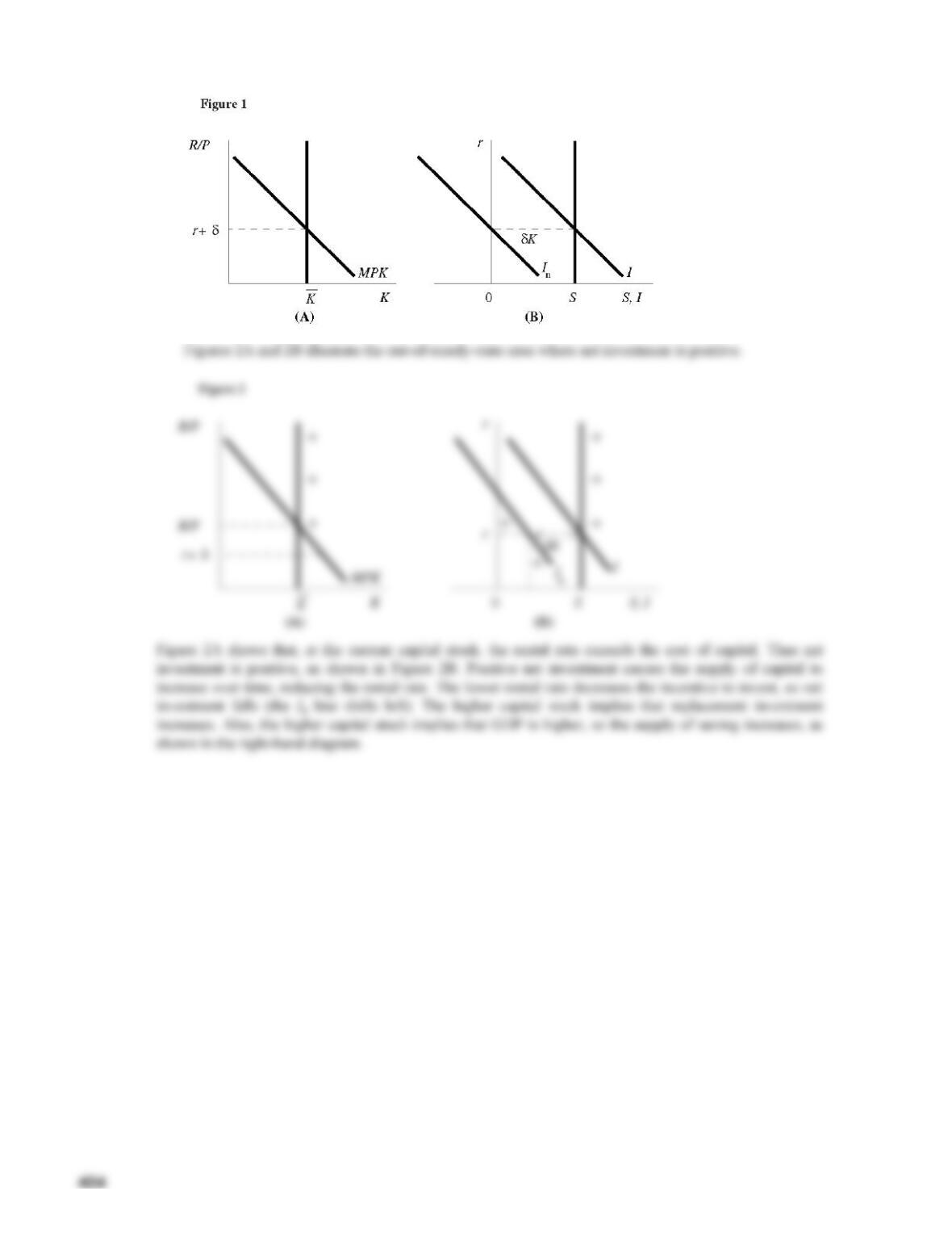
The rental price of capital goods is determined in the rental market for capital goods. Capital is
owned by the rental firms and is in fixed supply in the short run. Production firms demand
capital up to the point at which the marginal revenue from the last unit of capital equals the
marginal cost of that capital. This means that the production firm demands capital up to the point
at which the marginal product of capital (MPK) equals the real rental price (R/P). So the demand
The Cost of Capital
Rental firms choose how much capital to own and, therefore, how much new capital to acquire.
That is, they make the investment decision. For a rental firm, the benefit of owning a unit of
capital is that it can rent that capital to production firms and receive R/P. This rental price
implicitly has a time dimension—it is the price that production firms pay for the right to make
use of a unit of capital for some period of time (say, a year). Rental firms compare this benefit of
owning capital to the cost of a unit of capital over the same time period.
Suppose that PK is the price of a unit of capital (for example, a machine) in dollars.
Imagine that a rental firm borrows PK from the bank to purchase such a machine this year. At the
398 | CHAPTER 17 The Theory of Investment
(The term δ∆PK/PK, being the product of two small numbers, is very small and can be ignored.)
The cost of capital thus has three components. First, there is an interest cost, since the firm
must either borrow to purchase the unit of capital or else incur the opportunity cost of interest
forgone. The second is the depreciation cost, which results from the fact that the machine wears
out over the course of the year. The third component is the capital gain or loss—if the price of a
unit of capital increases over the period, then the rental firm makes a capital gain and the cost of
capital is lower. If we divide by the price level, we obtain the real cost of capital:
The Determinants of Investment
In deciding whether or not to purchase new capital, rental firms compare the revenue from a unit
of capital with the cost of a unit of capital. The difference between the two is its profit per unit of
capital, or profit rate:
Profit Rate = R/P – (PK/P) (r + δ).
Rental firms have an incentive to increase their stock of capital if the rental price exceeds the
cost of capital, and they have an incentive to decrease their stock of capital if the rental price is
less than the cost of capital. That is, if the rental price exceeds the cost of capital, then net
investment is positive. (Recall that net investment is investment in excess of that necessary to
replace depreciated capital.) From our analysis of the rental market for capital, we know that the
rental price of capital equals the marginal product of capital. We obtain finally that
Lecture Notes | 399
Investment depends negatively on the interest rate. Anything that increases the profit rate for any
given rate of interest (such as a technological innovation that raises the marginal product of
capital) shifts the demand for investment out.
Whenever net investment is positive, the capital stock is increasing and so the marginal
product of capital is falling. This reduces the profit rate and decreases the incentive to invest. In
the long run, increases in the capital stock thus drive the profit rate down to zero. When the
profit rate is zero, then net investment is also zero and the capital stock will be at its steady-state
level. In this case
Taxes and Investment
The incentive to invest is affected by provisions of the tax code. Corporate income taxes are
taxes levied on corporate profits. If profits were measured, as our theory suggests, by the
difference between the rental price of capital and the cost of capital, then the corporate income
tax would not distort the investment decision. But profit, for tax purposes, is defined somewhat
Case Study: Inversions and Corporate Tax Reform
When an American company merges with a foreign one and reincorporates abroad, the merger is
often referred to as a tax inversion. Although the reasons for mergers are many, an important one
is to take advantage of favorable tax treatment by some other nations. While companies and their
management should not be faulted for trying to increase their after-tax profits, the lost revenue to
the U.S. Treasury means that everyone else either has to pay higher taxes or receive fewer
government services. If tax inversions are indeed a problem, the fault should not be placed on
the business leaders who are meeting their responsibilities to shareholders, but instead should be
placed on the tax code, which provides incentives for these inversions.
The Stock Market and Tobin’s q
The economist James Tobin proposed a theory of investment that is distinct from, yet related to,
the neoclassical theory of investment. He suggested that net investment depends upon a number,
known as Tobin’s q:
!Supplement 17-1,
“The Short Run
and the Long
Run: Investment
and the Capital
Stock”
400 | CHAPTER 17 The Theory of Investment
the value of capital, as measured by the stock market, exceeds the cost of that capital. Therefore,
firms could increase their value by purchasing more capital.
If the marginal product of capital is greater than the cost of capital, firms earn profits on
the capital they own. Since these profits should ultimately influence the dividends paid out by
Case Study: The Stock Market as an Economic Indicator
As discussed in Chapter 10, the stock market is a leading indicator and so may help to predict
the future course of the economy. Changes in stock prices certainly do not correspond perfectly
with changes in GDP, but the two are related.
There are three reasons why stock prices and GDP fluctuate together:
Alternative Views of the Stock Market: The Efficient Markets
Hypothesis Versus Keynes’s Beauty Contest
Economists continue to debate the reasons for movements in stock market prices. One view,
known as the efficient markets hypothesis, assumes that a company’s stock price is a rational
valuation of a company’s value. According to this view, the stock market is informationally
efficient, so changes in the stock price of a company reflect new information about the future
prospects for the company. Any information already known about a company is incorporated
into investors’ valuation of its stock, and so only “news” should affect stock prices. Supporters
Financing Constraints
Firms may finance their investment either through retained earnings (that is, profits not
distributed as dividends) or by borrowing in financial markets. From the perspective of the
neoclassical theory of investment, these two are equivalent, since the theory assumes that firms
face no difficulty in borrowing. In reality, however, firms sometimes are limited in their ability
!Supplement 17-2,
“Asset Pricing I:
Why Do We
Care?”
!Supplement 17-3,
“Asset Pricing II:
Stock Prices and
Efficient Markets”
!Supplement 17-4,
“Asset Pricing III:
Bond Prices and
!Supplement 17-7,
“Financing
Constraints in
Japanese Firms”
17-2 Residential Investment
We now turn to the explanation of residential investment.
The Stock Equilibrium and the Flow Supply
At any time the stock of housing is fixed, so the supply of housing is fixed. The higher the
would then be analogous to rental firms in our previous theory. (Many modern apartment
complexes essentially take this form.) The existing supply of housing and the demand for
Changes in Housing Demand
If the demand for housing increases, perhaps because of population increases or economic
prosperity, the relative price of housing rises. This increases residential investment. Decreases in
the real interest rate also encourage residential investment, just as they encourage business fixed
investment. When the interest rate falls, mortgage rates fall, which increases the demand for
owner-occupied housing and encourages residential investment. Similarly, a fall in the interest
rate reduces the cost of capital to landlords who build and own rental accommodations.
Another key determinant of housing demand is credit availability. During the early to mid-
2000s, mortgage interest rates were low and mortgage loans were easy to obtain. Even
!Supplement 17-8,
“Taxes, Babies,
and Housing”
!Supplement 17-9,
“The Tax
Treatment of
Housing”
17-3 Inventory Investment
The third main component of investment is inventory investment. Although it is small in
magnitude, it is of great interest to economists because it is so volatile and thus accounts for a
substantial portion of GDP fluctuation.
Reasons for Holding Inventories
Firms hold inventories for four main reasons. The first is production smoothing: Although the
demand for a firm’s product may vary substantially over time, the firm might prefer to keep its
production relatively constant. Manufacturers of snow blowers may find it more efficient to
produce throughout the year and store snow blowers for sale in the winter, rather than attempt to
produce all their output in the winter months. Inventories may also serve as a factor of
How the Real Interest Rate and Credit Conditions Affect
Inventory Investment
Holding inventory is costly for firms. If an auto dealership holds a car on its lot for a month, it is
worse off than if it had sold the car, because it could then have placed the proceeds from the sale
in the bank and earned interest on them. So inventory investment, like the other types of
investment, depends negatively on the real interest rate. When real interest rates are high, firms
17-4 Conclusion
The models of this chapter reveal that all types of investment depend negatively on the real
interest rate, thus justifying the simple investment function adopted earlier in the textbook. They
!Supplement 17-10,
“The Importance of
Inventories”
!Supplement 17-11,
“Inventories and
Production
Smoothing”
!Supplement 17-12,
“Production
Smoothing and
Coordination
Failure”
!Supplement 2-6,
403
LECTURE SUPPLEMENT
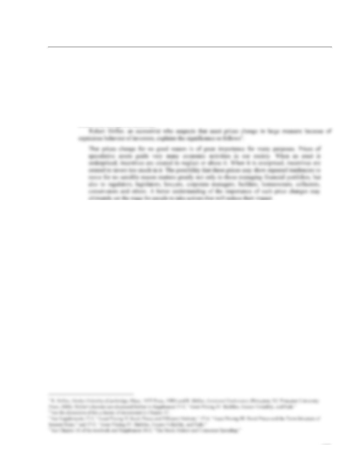
17-1 The Short Run and the Long Run: Investment and the Capital Stock
Saving, investment, and capital accumulation are discussed in a number of different places in the textbook.
The classical model presented in Chapter 3 of the textbook explains how the real interest rate brings
saving and investment into balance. The Solow growth model of Chapters 8 and 9 explains the long-run
process of capital accumulation. The neoclassical model of investment presented in Chapter 17 explains
the determinants of investment. How do all these models fit together?
Net investment thus equals the change in the capital stock.
The classical model assumes that the real rental price of capital is determined in the market for capital
goods, implying that
MPK = R/P.
The classical model also notes that the real interest rate adjusts to bring about equilibrium in the loanable-
funds market:
S = I(r).
The supply of saving is fixed over relatively short periods of time but depends in general on the level of
output and thus upon the existing capital stock. The neoclassical model of investment, meanwhile, argues
that net investment depends upon the difference between the rental price of capital and the cost of capital
405
ADVANCED TOPIC
17-2 Asset Pricing I: Why Do We Care?
One important area of macroeconomic study is that of asset pricing, that is, trying to explain the
equilibrium prices of various economic assets, such as stocks and bonds or houses. This involves the study
of financial markets and turns out to present a number of problems and puzzles that have not yet been fully
resolved. Yet it is an important area of macroeconomic inquiry because financial markets bring together
savers and investors in the economy. Our hope is that financial markets do a good job of directing
available loanable funds to those activities that are most profitable. Many economists do indeed believe
that financial markets operate efficiently and are an important aid to the smooth functioning of the
economy. Others are less sanguine and believe that irrational behavior in such markets may be a source of
shocks that disrupt the economy.
ultimately set the stage for people to take actions that will reduce their impact.
Much work on asset pricing focuses on the stock market. Macroeconomists are particularly interested
in the stock market for a number of reasons. First, movements in the stock market seem to be linked to
movements in aggregate economic activity. Second, as noted previously, the stock market brings together
savers and investors and thus helps guide the allocation of loanable funds to investment projects.2 Third,
the stock market, if it functions efficiently, provides information about investors’ expectations concerning
future economic performance. Macroeconomists are thus concerned by there being evidence of
inefficiency in the stock market.3
There is one observation suggesting that lack of efficiency in the stock market actually might not be
so serious. Most trading in the stock market is of existing shares, not new issues, and so has a less direct
influence on the allocation of resources. Even if stock market prices do change for no good reason, these
fluctuations in relative stock prices might then simply redistribute wealth from one set of gamblers to
another, and the consequences for the macroeconomy might not be that large. Aggregate movements in the
stock market still matter, however, because they represent changes in wealth, and wealth is a determinant
of consumption behavior.4
406
ADVANCED TOPIC
17-3 Asset Pricing II: Stock Prices and Efficient Markets
We discuss here some basic ideas about the pricing of a risky asset, focusing on the stock market.
Consider a situation in which investors can invest in a riskless asset, which pays a certain (real) rate of
return equal to r, or a stock, which pays an uncertain return.1 Ownership of a stock entitles the investor to
a stream of dividends. Dollars received in the future, however, are worth less than dollars today, because
holding return on the stock between period t and t + 1. The return on the stock consists of two
components: the dividend that it will pay and any capital gain or loss that arises because of a change in its
price. Thus, if pt is the price of the stock and dt+1 is the dividend, then
Return = Dividend + Capital Gain.
This is the basic equation for the pricing of a stock. It tells us that the price of a stock today depends upon
the dividend it will pay next period and the price of the stock next period.
An analogous equation will hold for the price of the stock next period:
ht=dt+1
pt
+pt+1−pt
pt
1+r
⎝
⎠
important implication of this is that changes in stock prices should come about only as a result of new
information. Thus, changes in stock prices should not be predictable on the basis of any currently available
information, for if they were, arbitragers would be able to make profits.5 The overall value of the stock
market, by extension, should reflect investors’ best predictions about the future profitability of all firms
(and hence, among other things, about the future state of the U.S. economy).
3 Supplement 17-6, “Asset Pricing V: The Capital-Asset Pricing Model,” considers how riskiness affects asset prices.
4 Different definitions of market efficiency are sometimes used depending upon exactly what information is reflected in the price of the stock.
5 This idea is sometimes loosely referred to as the random-walk theory: Stock prices should follow a random walk. See the discussion of rational-
expectations theories of consumption in Chapter 16 of the textbook for more discussion of random walks. See also S. LeRoy, “Efficient Capital
P
t=1
1+r
dt+1+1
1+r
2
dt+2+1
1+r
3
dt+3+1
1+r
4
dt+4+…,
408
ADVANCED TOPIC
17-4 Asset Pricing III: Bond Prices and the Term Structure of Interest Rates
The textbook speaks throughout of “the” interest rate. Yet we know that in the real world there are many
different interest rates. An important first observation is that the simplifying assumption of a single interest
rate is not badly misleading for much macroeconomic analysis, because different interest rates, broadly
speaking, tend to move together in practice.
return on assets depends upon their term to maturity is known as the term structure of interest rates.
As a preliminary to this, we consider the basic principles behind the pricing of a bond. A bond is an
asset that is described in terms of three basic characteristics: its term to maturity; the coupon that it pays
out each year; and its face value, which is the amount that it pays at maturity.3 Various assets exist that are
special cases: zero-coupon bonds, as the name suggests, pay only at maturity; perpetuities (or consols)
where C is the coupon payment. The sum of the infinite series in parentheses is simply 1/r, so we have
1 Stocks, Bonds, Bills, and Inflation 1988 Yearbook (Chicago: Ibbotson Associates, 1988), 77.
2See Supplement 17-6, “Asset Pricing V: The Capital-Asset Pricing Model.”
3 Bonds may, and often do, pay coupons more frequently than annually; for ease of presentation we here take the relevant time for analysis to be a
year.
=1
1+r
⎛
⎝
⎜⎞
⎠
⎟+1
1+r
⎛
⎝
⎜⎞
⎠
⎟
+1
1+r
⎛
⎝
⎜⎞
⎠
⎟
+…
⎧
⎨
⎪
⎩
⎪
⎫
⎬
⎪
⎭
⎪
C,
PDV =C
r
.
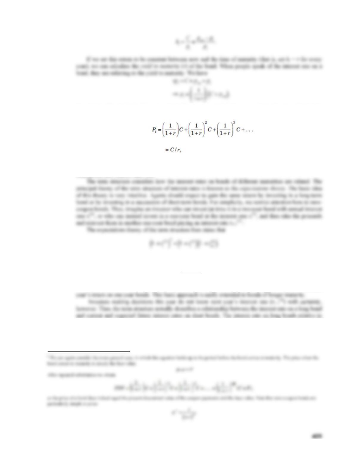
An equation like this holds for every period. By repeated substitution we can write the price of a bond at
time t as6
confirming that the price of the consol is indeed simply the coupon divided by the interest rate. The
important conclusion from this analysis is that bond prices and interest rates are inversely related: When
bond prices fall, interest rates rise.
As an approximation, we can write
In other words, the annual return on the two-year bond is approximately the average of this year’s and next
short bonds thus reflects agents’ expectations about future interest rates. To see this clearly, subtract rt
(1)
from both sides of the previous equation to get
r
t
(2) ≅r
t
(1) +r
t+1
(1)
2.


