According to this equation, the long rate will exceed the short rate if interest rates are expected to rise, and
the short rate will exceed the long rate if interest rates are expected to fall.
The expectations theory of the term structure explains theoretically why different interest rates tend to
r
t
(2) −r
t
(1) ≅r
t+1
(1) −r
t
(1)
2.
411
ADVANCED TOPIC
17-5 Asset Pricing IV: Bubbles, Excess Volatility, and Fads
There are a number of dramatic historical incidents known as speculative bubbles, where the price of an
asset rises and falls dramatically. One of the most famous is Tulipmania: In the Netherlands in the
seventeenth century, certain rare varieties of tulip bulbs sold at extraordinarily high prices. “For example,
a Semper Augustus bulb sold for 2,000 guilders in 1625, an amount of gold worth about $16,000 at $400
per ounce.”1 At the end of 1636 and the beginning of 1637, tulip bulb prices rose very rapidly and then
collapsed suddenly; two years later, bulbs were selling for less than 0.1 guilder. Another famous example
is the South Sea Bubble, during which the price of shares in the South Sea Company rose more than
eightfold between January and July 1720 and then fell back to about their original level in the next three
months.2 In these cases, it seems that the price of an asset changes not because of a change in the
fundamentals but because investors demand the asset in the anticipation of future price rises, brought
about in turn by more investors demanding the asset in the expectation of still further price rises, and so
on.3 These incidents make many economists skeptical of the purported efficiency of financial markets.
Further evidence of inefficiency is the observation that asset prices are much too variable to be
explained in terms of changes in fundamentals.4 The economist Robert Shiller is a strong proponent of this
view. Informal evidence of such excess volatility comes from the observation of major variation in asset
prices, such as the stock market crash of October 1987 or the recent movements in real estate prices in
some parts of the United States. Shiller and others have also provided more formal tests.
Shiller’s argument rests on a property of rational expectations and some simple statistics. He noted
that if the path of future dividends were known with certainty, then the perfect–foresight price of a stock
would be given by the present value of the stream of dividends.5 The actual price that investors are willing
to pay represents their prediction of this perfect–foresight price. If investors have rational expectations,
then the actual price will be the best possible forecast of the perfect–foresight price. The perfect–foresight
price then equals the actual price plus an unpredictable error term:
Yet another way to look for inefficiency in asset markets is to see whether there are unexploited profit
opportunities—ways to get something for nothing. Economists have looked for trading rules: simple rules
that could be mechanically applied and that would earn “above average” profits. Karl Case and Robert
Shiller suggested that a simple trading strategy could have exploited profit opportunities in the real estate
market.8 Bruce Lehmann showed that a contrarian strategy of taking short positions in winners (selling
stocks whose prices have recently increased) and long positions in losers (buying stocks whose prices have
recently fallen) would have made a profit over the period 1962–1986.9 Such findings are intriguing but do
not prove inefficiency. First, it has to be demonstrated that excess profits are large enough to overcome the
transactions costs of implementing the rule. Second, identifying a profitable trading rule on the basis of
past data is not a guarantee that it will work in the future. Third, as Donald McCloskey points out, such
researchers “must answer the American Question: if you’re so smart, why ain’t you rich?”10
Of course, some providers of investment advice do get rich by advising the market. That some do
succeed in outperforming the market is also apparently inconsistent with simple notions of market
efficiency. There are many such advisors operating, however, and so we should expect that some should
turn out to do well just by chance. The important question is, do we think that an investment service is
likely to be able to beat the market in the future if we observe that it has succeeded in so doing in the past?
85. One important question, analyzed by Sanford Grossman, concerns how different individuals’ private information is aggregated into the prices of
stocks. Grossman observes that for any individual investor the price of a stock provides an (imperfect) summary of the information of other agents.
Now suppose some investors (noise traders) trade for reasons unconnected with changes in information. If the demand of these traders falls, then

413
ADVANCED TOPIC
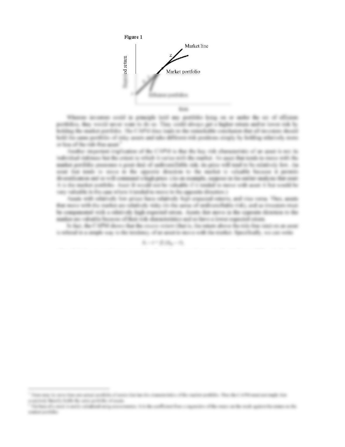
17-6 Asset Pricing V: The Capital–Asset Pricing Model
Different assets yield different returns.1 An important reason for this is that not all assets are equally risky.
In general, investors care not only about the expected return on an asset but also about its risk
characteristics.2 An important theory in financial economics, the capital–asset pricing model (CAPM),
seeks to explain how the return on an asset is connected to its riskiness.3 The basic idea is that to induce
agents to hold risky assets, it is necessary to compensate them with higher expected returns. But what
exactly determines the riskiness of an asset?
One natural supposition is simply that, the more variable is the return on an asset, the higher the return
that it must pay. This is not quite right because it ignores the very important observation that individuals in
general hold portfolios of assets and care only about their overall risk position, as determined by the
variability of their portfolio. By holding a number of different assets (that is, by diversification), investors
may end up with a portfolio that is less variable than any of the individual assets in their portfolio.
The CAPM starts off by describing assets in terms of both their average return and their variance. For
example, if asset A pays a return of 2 percent with probability 1/2 and 6 percent with probability 1/2, and
asset B pays either 0 percent or 8 percent, each with probability 1/2, then their expected or average return
is the same (4 percent), but asset B has higher variance. Now consider a portfolio that consists of 50
percent asset A and 50 percent asset B. Its expected return is simply the average of the expected return on
the two assets, which in this case is (trivially) 4 percent. The variance of this portfolio, however, depends
upon whether assets A and B tend to move in the same direction at the same time.
414
where hi is the expected return on stock i, hm is the expected return on the market portfolio, r is the risk–
free rate, and β measures the extent to which stock i covaries with the market.6 An asset that always moves
with the market has beta = 1; an asset that is unrelated to the market has beta = 0; an asset that moves in
the opposite direction to the market has a negative beta. The CAPM reveals that the excess return on an
asset is simply proportional to its beta. The CAPM is an example of a model that had a significant effect
on the world: Stock market analysts now routinely calculate the betas of different stocks.
A generalization of the CAPM, the consumption–based CAPM, suggests that the price of an asset
should depend not upon how it varies relative to the market, but on how it varies relative to consumption.
People hold assets as a means of saving, and people save to smooth their consumption. People will
therefore be particularly keen to acquire assets that offer a high return in times of relatively low
consumption. A stock will be particularly valuable, for example, if it tends to have a high return in
recessions, when consumption is relatively low.
ADDITIONAL CASE STUDY
17-7 Financing Constraints in Japanese Firms
A study by Takeo Hoshi, Anil Kashyap, and David Scharfstein provides some support for the idea that
financing constraints are important.1 They studied two types of Japanese firms. One set, known as the
keiretsu (industrial group), have close ties to large banks that finance their investment, so the firms find it
416
ADDITIONAL CASE STUDY
17-8 Taxes, Babies, and Housing
During the 1970s the United States experienced a nationwide boom in housing. The price of a new single–
family home relative to the CPI rose 30 percent from 1970 to 1980. Economists do not know with
certainty what caused the increase in housing prices during this period, but two hypotheses have been
proposed.
One hypothesis is that the rise in inflation and the failure of federal tax law to index for inflation
caused an increase in housing demand. The federal income tax subsidizes homeownership in two ways: It
does not require homeowners to pay tax on the imputed rent on their homes, and it allows homeowners to
deduct mortgage interest when computing their taxable income. Because the nominal interest rate on
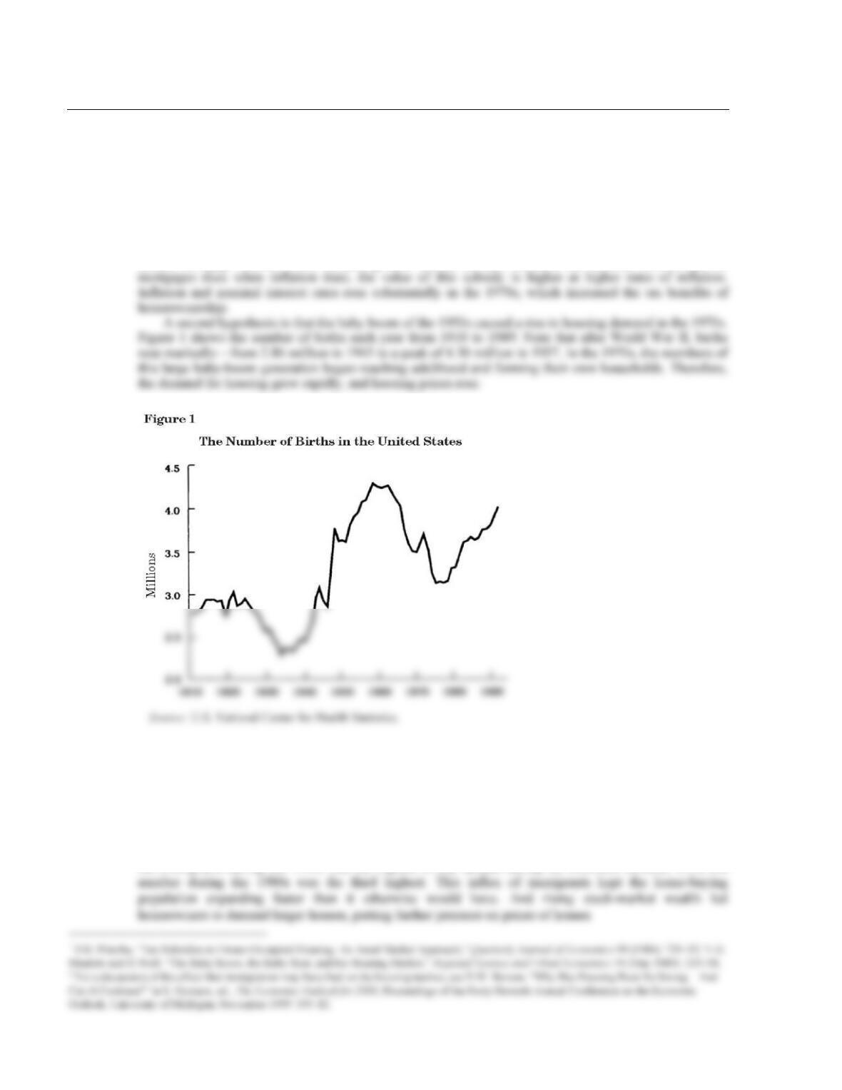
This baby–boom hypothesis suggested that the demand for new housing would fall during the 1990s.
In the 1970s births fell substantially, reaching a low of 3.14 million in 1973. In the 1990s this small baby–
bust generation reached adulthood. Some economists predicted that because of this slowdown in the
growth of the adult population, real housing prices would fall during the 1990s.1
In fact, housing prices continued to rise in the late 1990s—following a pause early in the decade in the
aftermath of the recession and the savings and loan crisis. Immigration and a rising stock market have
been pointed to as reasons why the earlier prediction of declining house prices was wrong.2 The number of
net immigrants during the 1990s was the highest of any decade during the twentieth century, while the
417
LECTURE SUPPLEMENT
17-9 The Tax Treatment of Housing
Chapter 17 discusses the effects of tax laws on business fixed investment. Tax laws also have effects on
residential investment. In this case, however, their effects are nearly the opposite. Rather than
discouraging investment, as the corporate income tax does for businesses, the personal income tax
subsidizes households to invest in housing.
A homeowner can be viewed as a landlord who also rents her own house. But she is a landlord with
special tax treatment. The United States does not tax her on the imputed rent (the rent she “pays” herself),
yet it allows her to deduct mortgage interest. Thus, when computing her taxable income, she can subtract
CASE STUDY EXTENSION
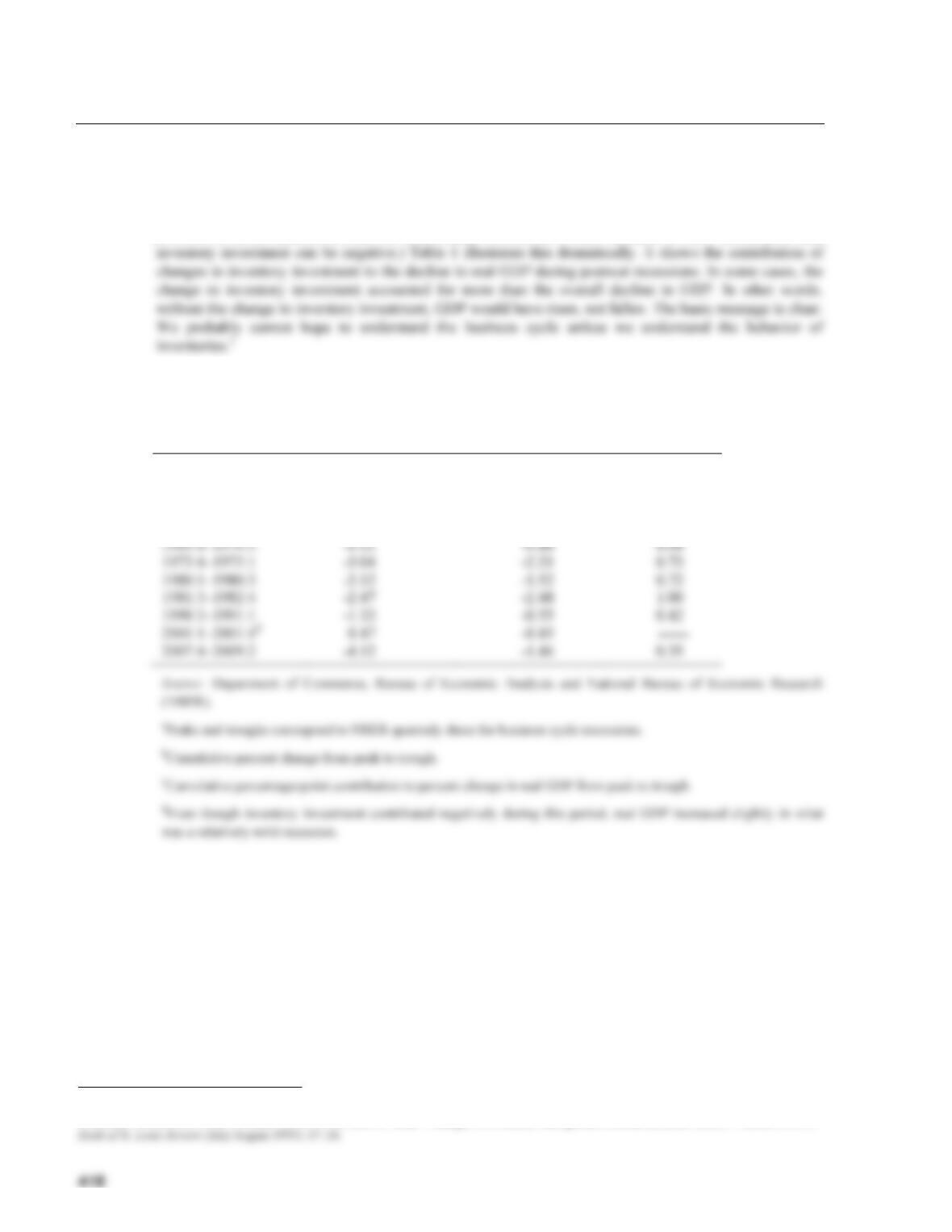
17-10 The Importance of Inventories
Inventory investment is a very small component of GDP. For example, in 2011, GDP was $17,421 billion,
and gross private investment was $2,856 billion, whereas inventory investment was a mere $90 billion.
Nevertheless, the behavior of inventories may be very important for macroeconomics, because
fluctuations in inventories account for a substantial fraction of overall variation in GDP. (Remember that
Table 1 Inventory Investment and Postwar Recessions
Cycle Peak to
Trougha
Change in Real
GDPb
Contribution from
Inventory
Investmentc
Contribution
as a Share of
Decline in GDP
1948:4–1949:4
–1.43
–3.01
2.10
1953:2–1954:2
–2.36
–1.39
0.59
1957:3–1958:2
–2.85
–1.16
0.41
1960:2–1961:1
–0.28
–0.94
3.29
1969:4–1970:4
–0.11
–0.88
8.08
1973:4–1975:1
–3.04
–2.21
0.73
1981:3–1982:4
–2.47
–2.48
1.00
1990:3–1991:1
–1.32
–0.55
0.42
–0.45
1 For a more detailed analysis, see A. Blinder and L. Maccini, “Taking Stock: A Critical Assessment of Recent Research on Inventories,” Journal of
Economic Perspectives 5, no. 1 (Winter 1991): 73–96; and D. Allen, “Changes in Inventory Management and the Business Cycle,” Federal Reserve
ADDITIONAL CASE STUDY
17-11 Inventories and Production Smoothing
The production–smoothing model does not do a good job of explaining inventories: Output and sales move
closely together. The standard production–smoothing model suggests that production should be less
variable (smoother) than sales. The economist Alan Blinder and others have documented that this is not
the case. For example, Blinder compares the variance of sales to the variance of production for various
manufacturing industries. For manufacturing industries as a whole, he finds that the ratio
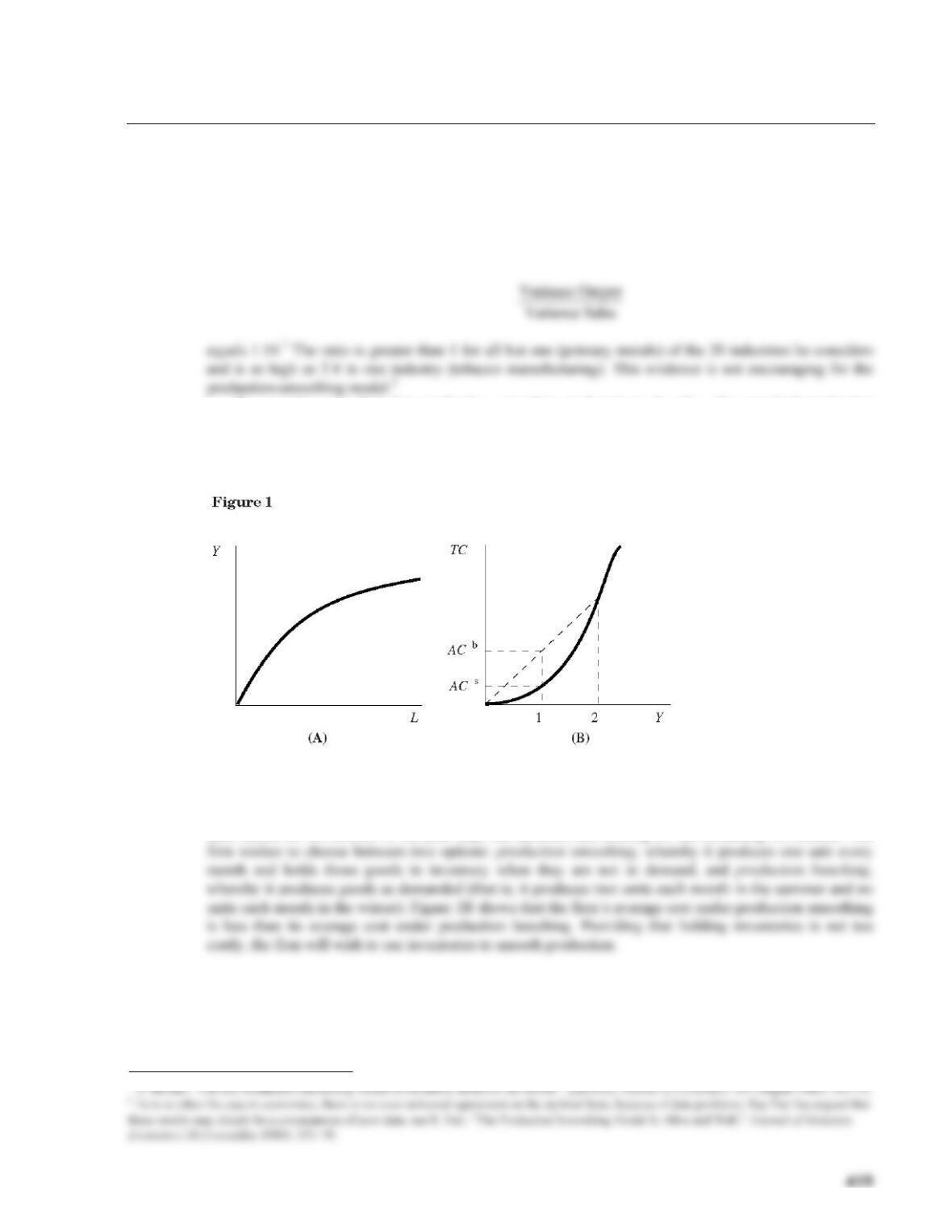
To see why, note first that production smoothing is based on the idea of a standard production
function exhibiting diminishing marginal product. Think, for example, of a firm with a given stock of
capital choosing how much labor to hire. Its production function takes the familiar form shown in Figure
1A.
Diminishing marginal product implies that each extra unit of output requires more and more labor. The
firm’s total cost curve is illustrated in Figure 1B: It shows total cost as a function of output.
Now suppose that this firm faces seasonal demand. For simplicity, suppose it sells two units of output
each month for six months of the year (say, the summer) and nothing for the remaining six months. The
1 A. Blinder, “Can the Production Smoothing Model of Inventory Behavior Be Saved?” Quarterly Journal of Economics 101 (August 1986): 431–53.
420
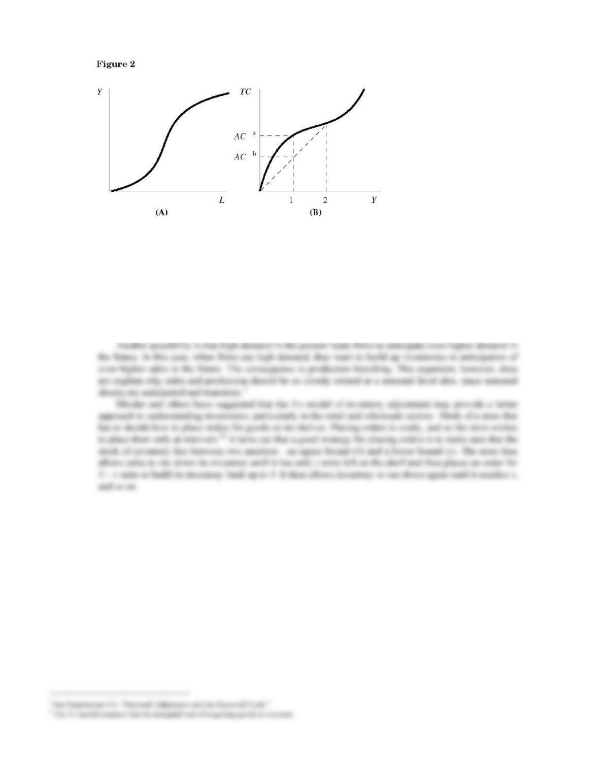
We arrive at a very different conclusion if the firm’s production function displays increasing returns
to scale over some range. In this case, large–scale production may be more efficient than small–scale
production. A production function exhibiting increasing returns (initially) is shown in Figure 2A; the
associated total cost curve is shown in Figure 2B. As Figure 2B shows, it is now better for the firm to
engage in production bunching rather than production smoothing.
Greater variability of production than of sales can be reconciled with more standard assumptions on
technology. One possibility is that firms face highly variable costs, although this is not very satisfactory
because, as Blinder notes, it “comes perilously close to assuming the conclusion (production is variable
because it is variable!).”
ADDITIONAL CASE STUDY
17-12 Production Smoothing and Coordination Failure
A striking example of production smoothing occurred in the automobile industry in the 1930s.1 Up to
1935, production was extremely volatile in the auto industry: Most manufacturers introduced new models
at the automobile shows in New York and Chicago in mid–January, while most demand was concentrated
in the spring, with the onset of good weather. As a consequence, most production was concentrated in a
422
ADVANCED TOPIC
17-13 The Multiplier–Accelerator Model
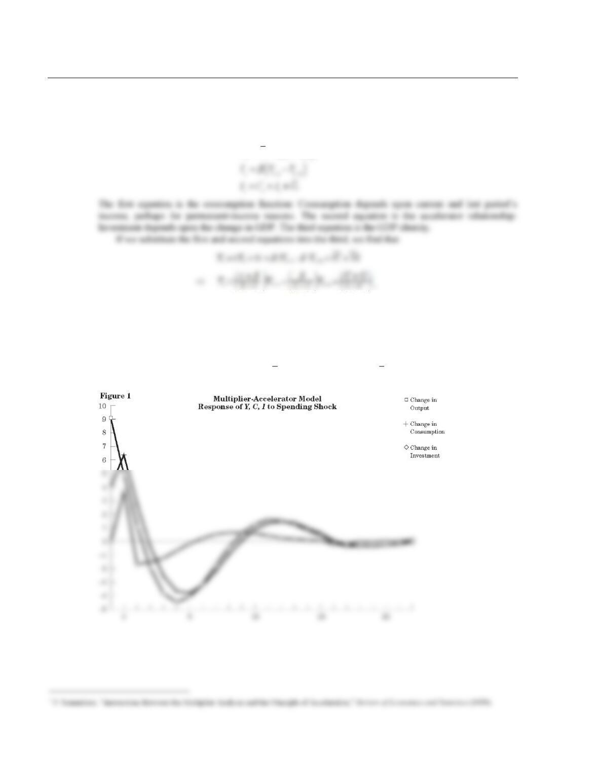
The Nobel Prize–winning economist Paul Samuelson combined the idea of the accelerator relationship in
investment and the multiplier from consumption to develop a model of cyclical behavior.1 Here is a simple
example of his multiplier–accelerator model:
Now suppose that there is a shock to this economy—for example, government spending is temporarily
increased at time t = 1. Output rises in period one and rises further in period two as a result of the
multiplier effect of increased consumption. The increase in output between periods one and zero
encourages investment—the accelerator effect. This increase in investment, in turn, increases income and
consumption. Output does not keep increasing at the same rate, however. As the change in output declines,
investment falls. The economy may exhibit cycles as it adjusts to steady state. Figure 1 shows an example
of this adjustment for the following model: = 10; c = 0.45; β = 0.4; = 10; ∆G = 5.
Ct=C+c Yt+Yt–1
( )
C
G
LECTURE SUPPLEMENT
17-14 Additional Readings
For a very readable discussion of theory and facts about inventory investment, see Alan Blinder and Louis
1987): 73–86.
There is an extensive literature on asset pricing and stock market volatility. The Economist has a
“Schools Brief” on the capital–asset pricing model (February 2, 1991): 72–73; discussions of this model