398 CHAPTER 16 | Fiscal Policy
Appendix
A Closer Look at the Multiplier (pages 979–983)
Learning Objective: Apply the multiplier formula.
When economists forecast the effect of a change in spending or taxes, they often rely on econometric
models.
An Expression for Equilibrium Real GDP
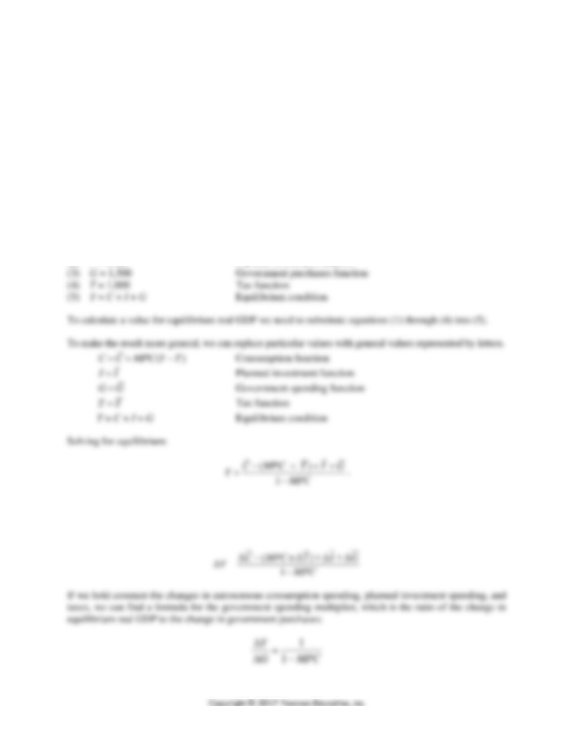
We can write a set of equations that includes the key macroeconomic relationships we studied in this and
previous chapters. We assume that taxes, T, do not depend on the level of real GDP, Y. There are no
government transfer payments to households, and there are no exports or imports. The numbers represent
billions of dollars.
(1) C = 1,000 + 0.75(Y – T) Consumption function
(2) I = 1,500 Planned investment function
A Formula for the Government Purchases Multiplier
To find a formula for the government purchases multiplier, rewrite the last equation for changes
in each variable, rather than levels:
CHAPTER 16 | Fiscal Policy 399
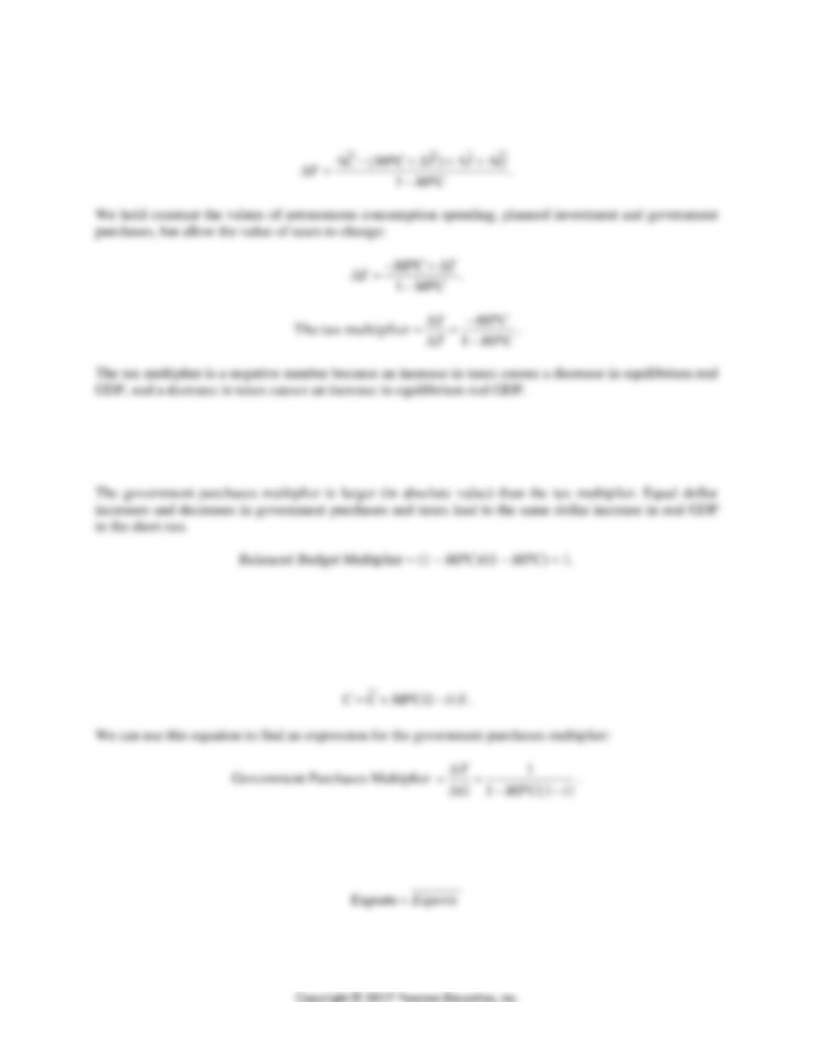
A Formula for the Tax Multiplier
To derive a formula for the tax multiplier start with the equation:
The “Balanced Budget” Multiplier
We can use the formulas for the government purchases multiplier and the tax multiplier to calculate the
net effect of increasing government purchases by the same amount as taxes are increased.
The Effects of Changes in Tax Rates on the Multiplier
We consider the effect of a change in the tax rate, as opposed to a change in a fixed amount of taxes.
Changing the tax rate changes the value of the multiplier. In general, an increase in income can be
multiplied by (1 – t) to find the change in disposable income, where t is the tax rate. We can rewrite the
consumption function as:
The Multiplier in an Open Economy
We can consider the case of an open economy by including net exports in our analysis. We assume that
exports are autonomous.
400 CHAPTER 16 | Fiscal Policy
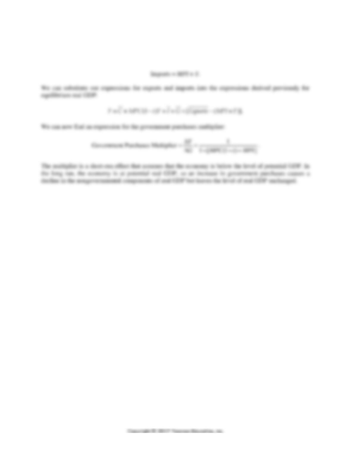
Imports will increase as real GDP increases because households will spend some portion of an increase in
income on imports. The marginal propensity to import (MPI) is the fraction of an increase in income that
is spent on imports:
CHAPTER 16 | Fiscal Policy 401
Solutions to End-of-Chapter Exercises
16.1
What Is Fiscal Policy?
Learning Objective: Define fiscal policy.
Review Questions
1.1 Fiscal policy refers to changes in federal government purchases and taxes that are intended to
1.2 Automatic stabilizers refer to government spending and taxes that automatically increase or
decrease along with the business cycle. Two examples of automatic stabilizers are unemployment
1.3 Federal purchases refer to federal spending where the federal government receives a good, such
as an aircraft carrier, or a service, such as the services of an FBI agent, in return. Federal
Problems and Applications
1.4 Fiscal policy refers to changes in federal government purchases and taxes that are intended to
achieve macroeconomic policy objectives, such as high employment, price stability, and high
1.5 a. Not part of fiscal policy because the action is not intended to affect the national economy.
b. Not part of fiscal policy, but is instead an example of monetary policy.
402 CHAPTER 16 | Fiscal Policy
e. Not part of fiscal policy, but is an example of environmental policy.
1.6 Not necessarily. Federal income tax revenue changes as tax rates change and as incomes change.
A reduction in tax revenue can be the result of lower tax rates or lower incomes. For example,
1.7 Birth rates were high between the end of World War II and the early 1960s (the so-called “baby
boom” period) and much lower in the years before and after the baby boom. As a result, there are
more baby boomers than there are members of either the generation born before or the generation
16.2
The Effects of Fiscal Policy on Real GDP and the Price Level
Learning Objective: Explain how fiscal policy affects aggregate demand and how the
government can use fiscal policy to stabilize the economy.
Review Questions
2.1 An expansionary fiscal policy is a decrease in taxes or an increase in government purchases
intended to increase aggregate demand. A contractionary fiscal policy is an increase in taxes or a
Problems and Applications
2.3 You should disagree. A decrease in taxes increases aggregate demand and real GDP and an
increase in taxes reduces aggregate demand and real GDP. The statements are incorrect because
CHAPTER 16 | Fiscal Policy 403
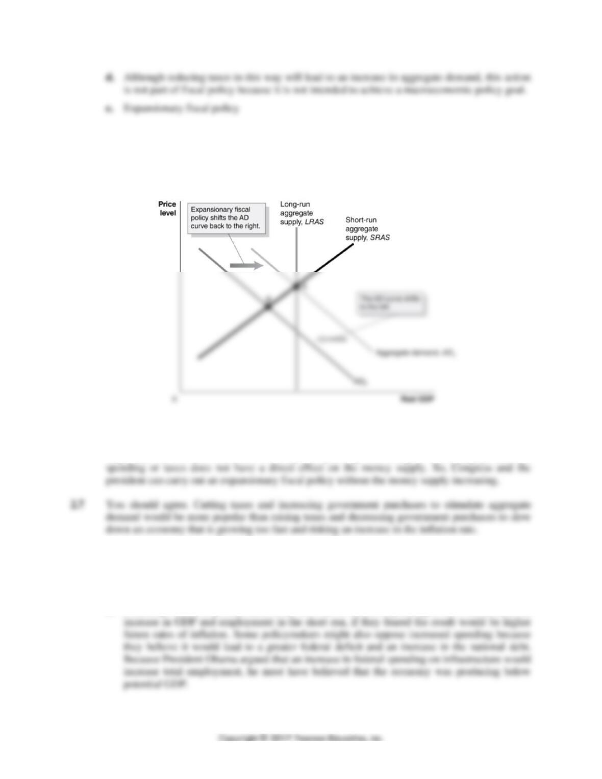
2.5 Equilibrium is initially at the intersection of LRAS, SRAS and AD1 (point A). The aggregate
demand curve shifts to the left from AD1 to AD2 and short-run equilibrium moves to point B.
Congress and the president can engage in an expansionary fiscal policy by increasing government
spending or reducing taxes (or both), to shift AD to the right, from AD2 back to AD1.
2.6 The purpose of expansionary fiscal policy is to increase aggregate demand either by having the
government directly increase its own purchases or by cutting taxes to increase household
disposable income and, therefore, consumption spending. Increasing or decreasing government
2.8 a. Increases in federal spending will increase real GDP and employment in the short run if the
economy is producing at less than its potential output and has some cyclical unemployment.
If the equilibrium rate of real GDP is equal to or greater than its potential rate of GDP then
increases in federal spending will result in crowding out and increases in the price level.
b. Federal government policymakers may not want to increase spending, even if the result is an
404 CHAPTER 16 | Fiscal Policy
16.3
Fiscal Policy in the Dynamic Aggregate Demand and Aggregate
Supply Model
Learning Objective: Use the dynamic aggregate demand and aggregate supply model
to analyze fiscal policy.
Review Questions
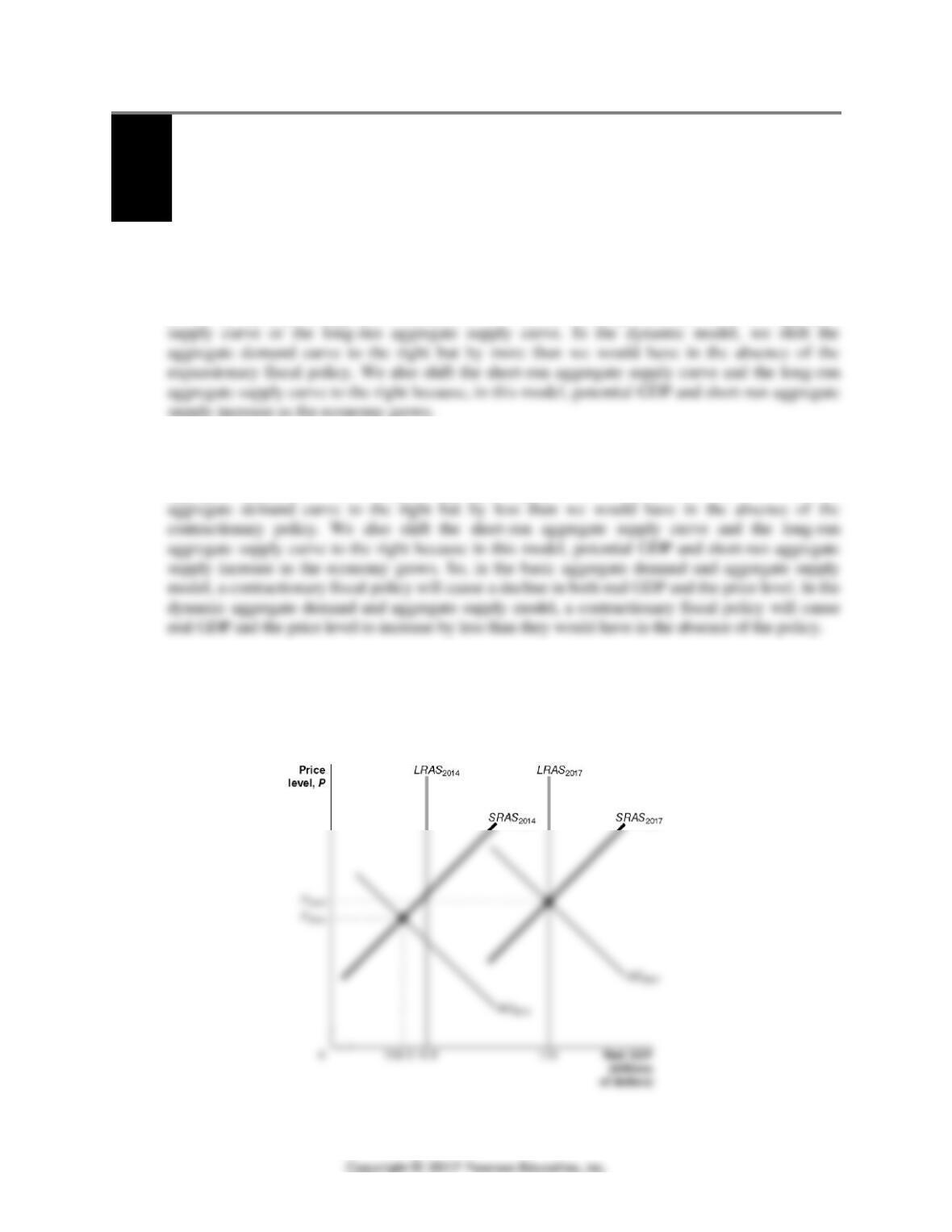
3.1 In the basic aggregate demand and aggregate supply model, we illustrate an expansionary fiscal
policy by shifting the aggregate demand curve, while not shifting either the short-run aggregate
3.2 In the basic aggregate demand and aggregate supply model, we illustrate a contractionary fiscal
policy by shifting the aggregate demand curve to the left, while not shifting either the short-run
aggregate supply curve or the long-run aggregate supply curve. In the dynamic model, we shift the
Problems and Applications
3.3 a. It is possible for the economy to produce more than its potential GDP, but a rate of output
that high would not sustainable in the long run.
b.
CHAPTER 16 | Fiscal Policy 405
3.4 a. The value of real GDP will be $18.2 trillion, and the price level will be 117.
b. The government can conduct an expansionary fiscal policy by increasing government
purchases or decreasing taxes.
3.5 a. Because real GDP is below potential GDP in 2019, Congress and the president should use
expansionary fiscal policy to keep real GDP at its potential level. Expansionary policy
c.
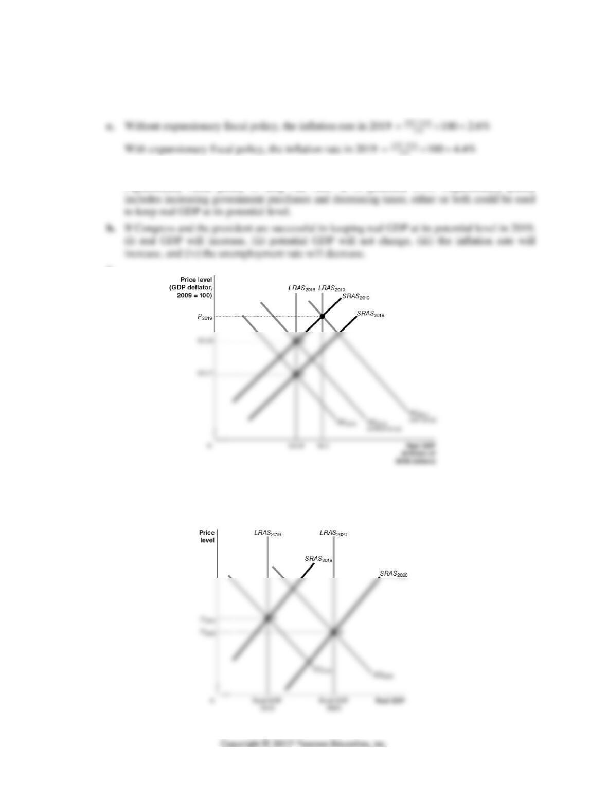
3.6 The economy does not have to be in a recession during 2020 for deflation to take place. As is
shown on the following graph, aggregate demand increases from 2019 to 2020, but the shift to the
right in short-run aggregate supply is greater than the shift to the right in aggregate demand,
resulting in an increase in real GDP but also a decrease in the price level (point A to point B).
406 CHAPTER 16 | Fiscal Policy
16.4
The Government Purchases and Tax Multipliers
Learning Objective: Explain how the government purchases and tax multipliers work.
Review Questions
4.1 A $1 increase in government purchases initially increases real GDP and national income by $1.
4.2 The government purchases multiplier is the ratio of the change in equilibrium real GDP to the
Problems and Applications
4.4 The Caldecott Tunnel and similar construction projects represent an increase in government
4.5 Keynes described the multiplier effect. By repercussions, he meant the rounds of spending and
4.6 a. To bring the economy to equilibrium at potential GDP, government purchases need to be
increased by the needed change in real GDP divided by the government purchases multiplier:
4.7 The statement is incorrect because it ignores the multiplier effect. Equilibrium real GDP would
decrease by more than $300 billion following a $300 billion decrease in government purchases or
CHAPTER 16 | Fiscal Policy 407
4.8 a. The size of the government purchases multiplier is different from the size of the tax
multiplier. So, the size of the multiplier depends on the type of fiscal policy—changes in
government purchases or changes in taxes—that is used.
b. When real GDP is close to potential GDP, an increase in government purchases or a cut in
16.5
The Limits to Using Fiscal Policy to Stabilize the Economy
Learning Objective: Discuss the difficulties that can arise in implementing fiscal policy.
Review Questions
5.1 Monetary policy can be changed more quickly than fiscal policy. The Federal Open Market
Committee can change monetary policy at any of its meetings, which are scheduled to occur eight
Problems and Applications
5.3 a. This outcome will most likely occur if investment spending is crowded out because
5.4 Many economists believe that consumers base their spending decisions on their permanent
income rather than their current income. A one-time tax rebate affects households’ current
5.5 a. The government purchases multiplier can have a value less than 1 if an increase in
government spending results in a decline in private expenditures: private investment
408 CHAPTER 16 | Fiscal Policy
b. In evaluating the effects of an expansionary fiscal policy, an estimate of the size of the
5.6 Recessions accompanied by a financial crisis involve more than simply a decrease in aggregate
expenditure leading to a recession. Recessions accompanied by a financial crisis involve credit
crunches where firms and households have difficulty obtaining loans to finance investment
5.7 An expansionary fiscal policy will tend to cause the equilibrium rate of interest to increase. An
expansionary monetary policy will cause the equilibrium rate of interest to decrease. An
5.8 a. “Low government borrowing costs” refers to the low interest rates that prevailed on U.S.
Treasury bonds and on government bonds in other countries in 2014 and 2015. If
infrastructure investments were made by the government at this time, the cost to borrow
funds to finance the investments would be lower than they would be if interest rates were
higher.
b. A policy lever refers to a policy action. The Fed and other central banks had been trying
various monetary policy actions, including quantitative easing, without managing to complete
16.6
Deficits, Surpluses, and Federal Government Debt
Learning Objective: Define federal budget deficit and federal government debt and
explain how the federal budget can serve as an automatic stabilizer.
Review Questions
6.1 When real GDP falls below potential GDP, households and firms pay less in taxes to the federal
government and the federal government makes more transfer payments to the unemployed. These
CHAPTER 16 | Fiscal Policy 409
6.2 The cyclically adjusted budget deficit or surplus measures what the budget deficit or surplus would
be if the economy were at potential GDP. A recession would decrease government tax revenues and
increase government spending on transfer payments, which would lead to a federal budget deficit.
6.3 Balancing the government’s budget during a recession would require raising taxes or reducing
government purchases. These actions would reduce aggregate demand and make the recession
Problems and Applications
6.5 Josh Zumbrun and Nick Timiaos provided the following responses to these questions:
a. “A lot of people want to make this analogy between individuals and the government.
Economists think this is a really bad analogy. The U.S. government is 238 years old and isn’t
planning to retire one day. If you were going to live forever, and bring in revenue forever,
6.6 An excessive budget deficit would be a budget deficit that would be unsustainable in the long run
and raise the risk that the government could default on its debt. Judging whether a budget deficit
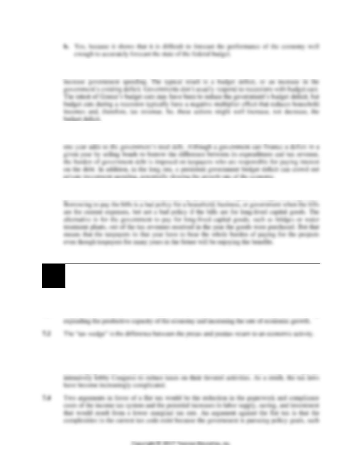
6.7 Balancing the federal government’s budget in 1932 was not a good idea because the economy
was in the midst of the Great Depression. Increasing taxes and cutting government purchases
would reduce aggregate demand and further reduce real GDP.
410 CHAPTER 16 | Fiscal Policy
6.9 When a country enters a recession, tax revenues decrease as household incomes and business
profits fall. Government payments for unemployment benefits and other transfer programs
6.10 A budget deficit is a situation in which the government’s expenditures are greater than its tax
revenue. Government debt is the total value of a government’s outstanding bonds. A deficit in
6.11 There is some truth in the columnist’s argument, but he is overlooking a key reason that the
government borrows to finance infrastructure projects, such as repairs to bridges and highways.
16.7
The Effects of Fiscal Policy in the Long Run
Learning Objective: Discuss the effects of fiscal policy in the long run.
Review Questions
7.1 Supply-side economics refers to fiscal policy actions intended to have long-run effects by
Problems and Applications
7.3 The tax laws are used for many purposes, including encouraging certain activities and
discouraging others. Every year, businesses, labor unions, charities, and many other groups
CHAPTER 16 | Fiscal Policy 411
7.5 The increase in marginal tax rates would cause both aggregate demand and long-run aggregate
supply to decline relative to what they would have been in the absence of the tax increase. As a
7.6 A cut in marginal tax rates increases the incentives to work, save, invest, and start a business. If
Real-Time Data Exercises
D16.1 The output gaps as a percentage of potential GDP as reported in The World Economic Outlook,
October 2013 for Japan, the United Kingdom, and the United States are:
Country
2013
2014
2015
2016
2017
2018
Japan
−0.938
−0.491
−0.256
−0.078
0.013
0.046
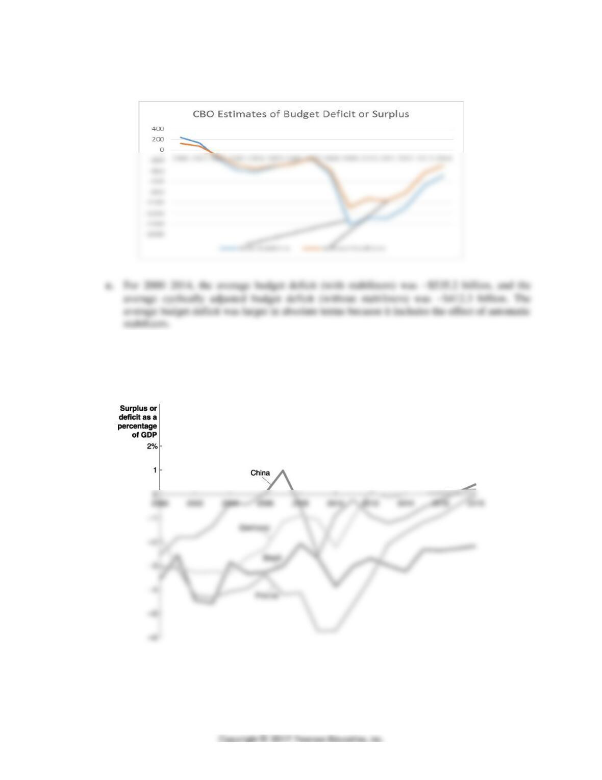
D16.2 a. Automatic stabilizers do not operate when the economy is at potential GDP, so the cyclically
adjusted budget deficit or surplus is not affected by automatic stabilizers. The actual budget
deficit or surplus does not assume that the economy is at potential GDP as the cyclically
412 CHAPTER 16 | Fiscal Policy
b. See graph below.
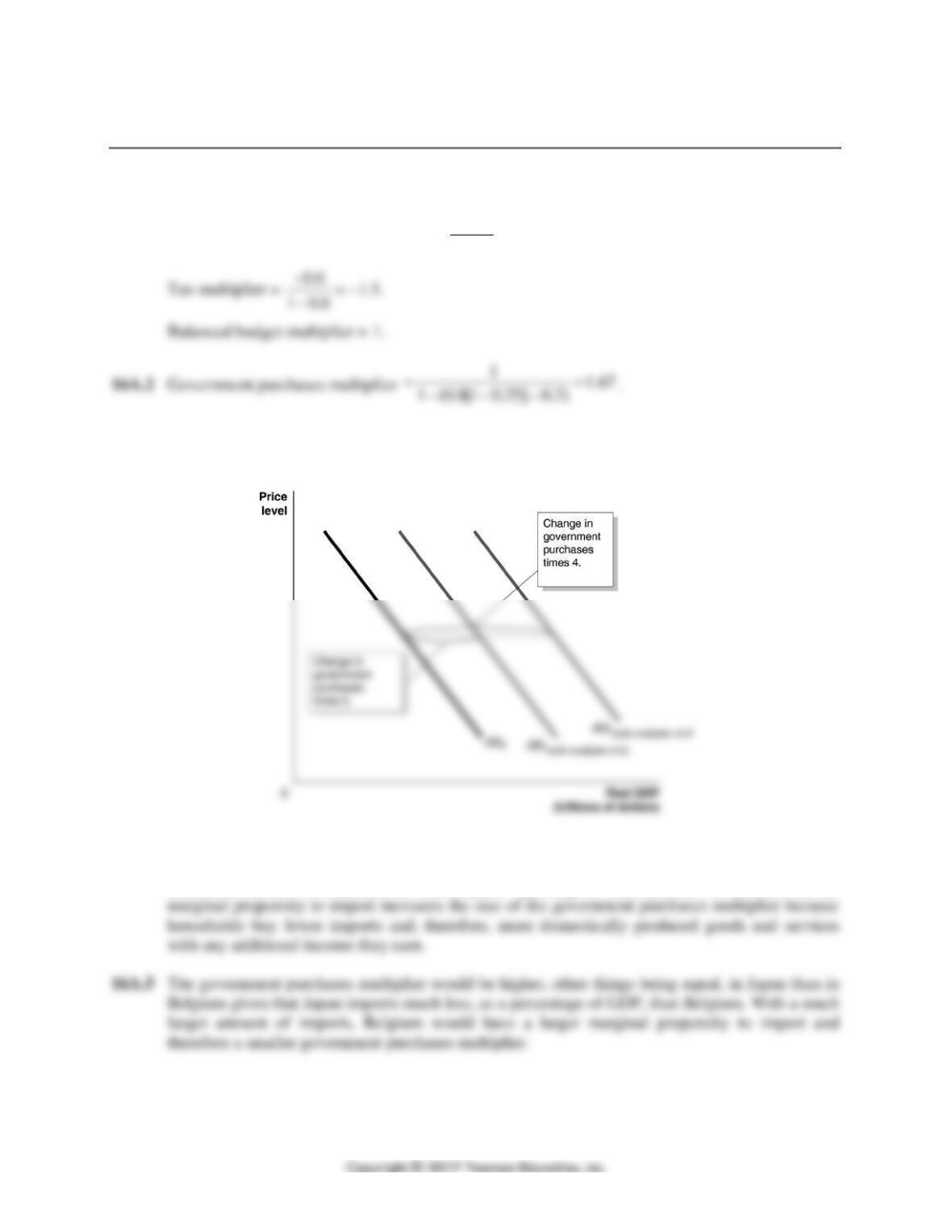
D16.3 a. France relied on discretionary fiscal policy the most in response to the financial crisis of 2008
and 2009. Of the four countries, France had the highest cyclically adjusted budget deficit as a
percent of potential GDP in 2008 of −4.129 percent and in 2009 of −5.721 percent.
b. From 2013 to 2018, Brazil is expected to have the most expansionary discretionary fiscal
policy as it is expected to have the highest cyclically adjusted budget deficits.
CHAPTER 16 | Fiscal Policy 413
Solutions to Chapter 16 Appendix
Problems and Applications
16A.1 Government purchases multiplier =
1
1 0.6−
= 2.5.
16A.3 The aggregate demand curve will shift to the right by the change in government purchases
multiplied by the government purchases multiplier.
16A.4 An increase in the tax rate decreases the size of the government purchases multiplier because it
increases the amount of taxes households must pay on any additional income they earn and,
therefore, reduces the amount of consumption spending in each period. A decrease in the