Chapter 16 Economic Analysis in the Service Sector
Cost–Effectiveness Analysis
Valuation of Benefits and Costs
16.1
(a) • User’s benefits:
– Prevention (or retardation) of highway corrosion: resulting in lower highway
maintenance cost. This lower maintenance cost implies lower users’ taxes
on gasoline, and so forth.
(b) The state of Michigan may declare certain sections of highway for
experimental purpose. CMA may be used exclusively for a designated area
16.2 Open end question (Not provided)
16.3 Open end question (Not provided)
Benefit–Cost Analysis
16.4
B=$786,000(P/A,8%,15) +$200,000(P/F,8%,15)
= $6,790,799
16.5
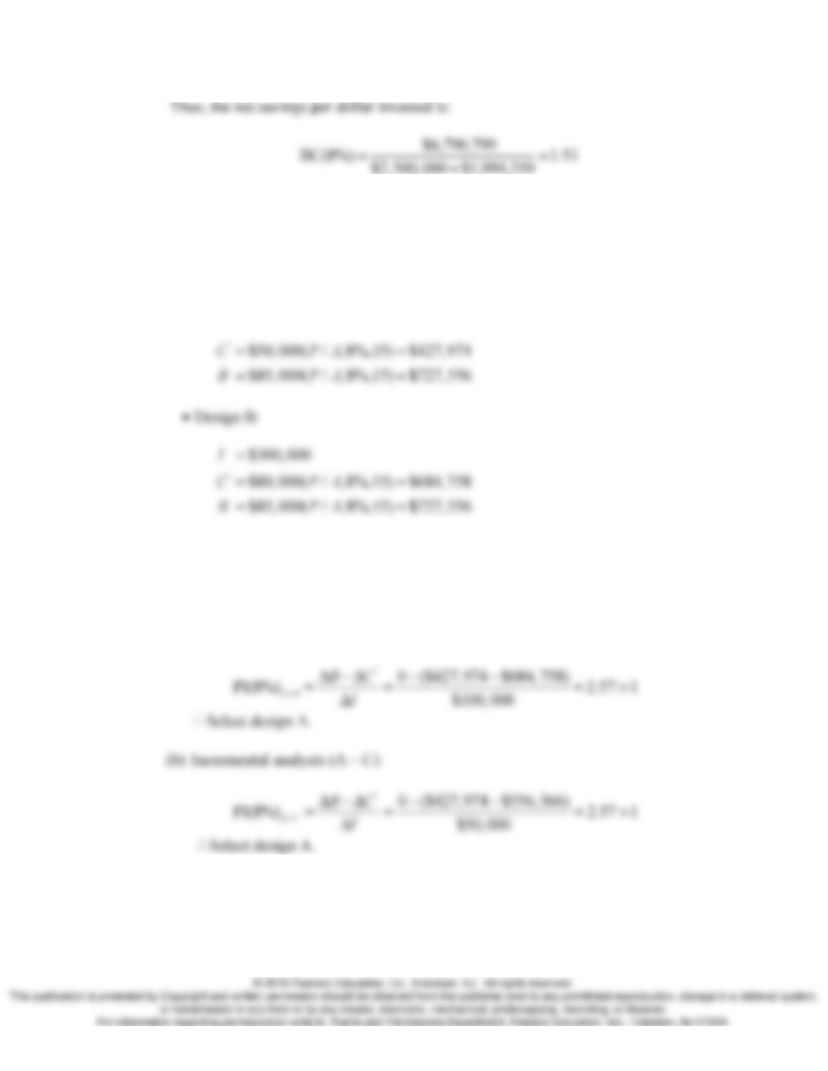
(a)
BC(i)
analysis:
•Design A:
$400,000
I
=
•Incremental analysis: Fee collections in the amount of $85,000 will be the
same for both alternatives. Therefore, we will not be able to compute the
( )BC i
ratio. If this happens, we may select the best alternative based on either
the least cost
‘
( )I C+
criterion or the incremental
PI( )i
criterion. Using the
incremental
PI( )i
criterion,
16.6
16.7
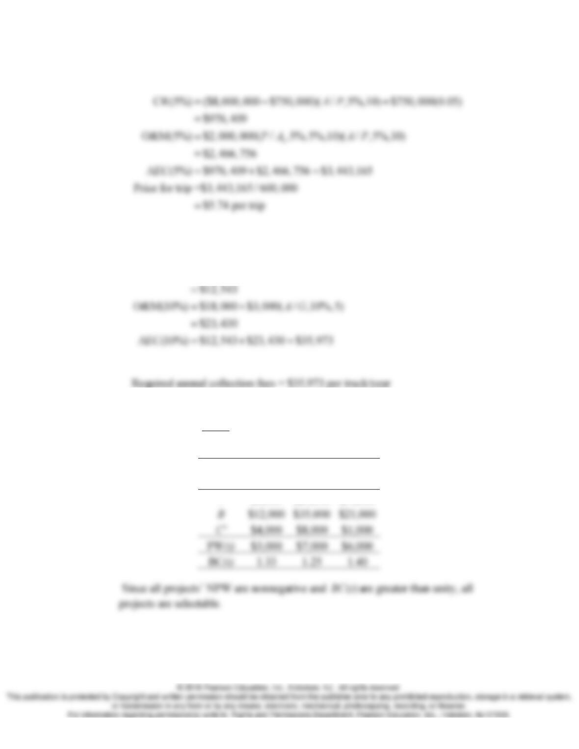
CR(10%) ($55,000 $12,000)( / ,10%,5) $12,000(0.10)
AP
=−+
16.8
(a) From
BC( ) B
i
IC
=′
+
Projects
A1
A2
A3
I
$5,000
$20,000
$14,000
$12,000
$35,000
$21,000
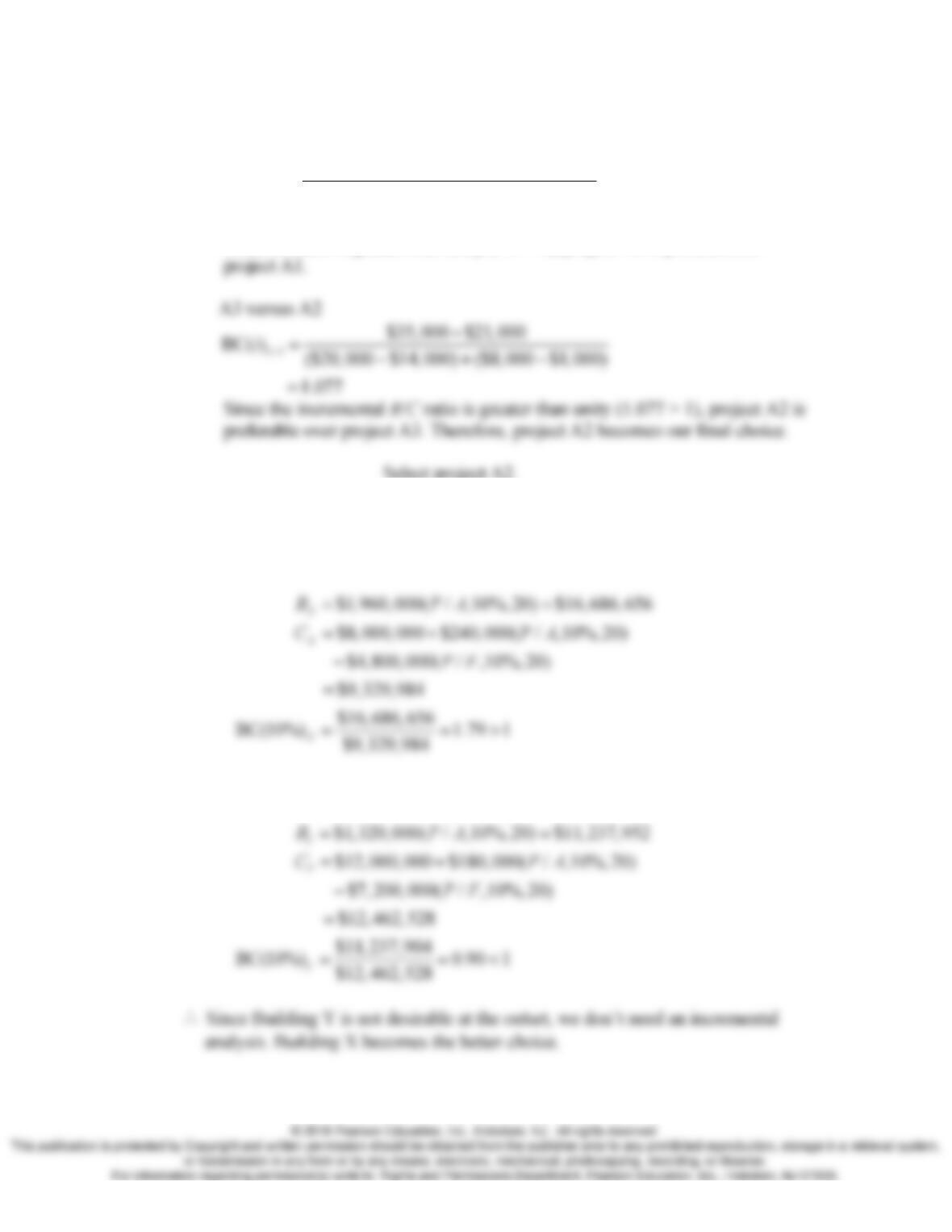
(b)
A1 versus A3
31
$21,000 $12,000
BC( ) ($14,000 $5,000) ($1,000 $4,000)
1.5
i−
−
=
−+−
=
Since the ratio is greater than unity (1.5 > 1), project A3 is preferable to
Select project A2.
16.9
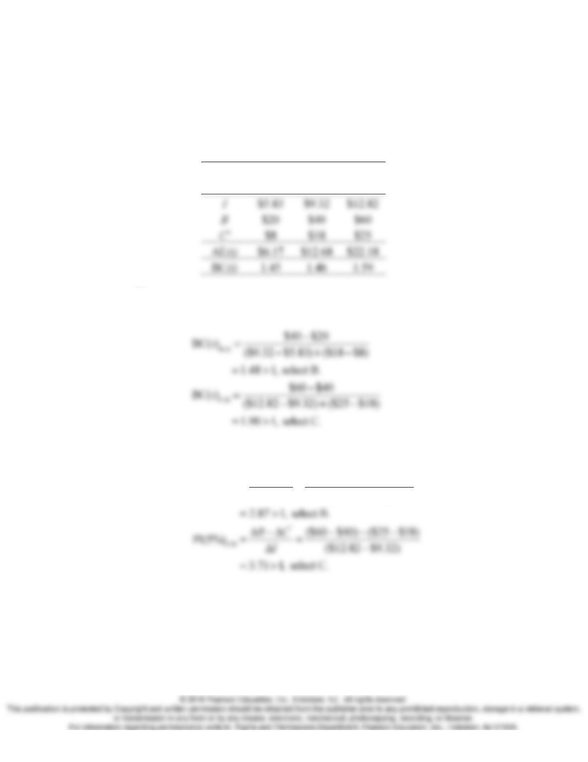
•Building X:
•Building Y:
16.10
(a)
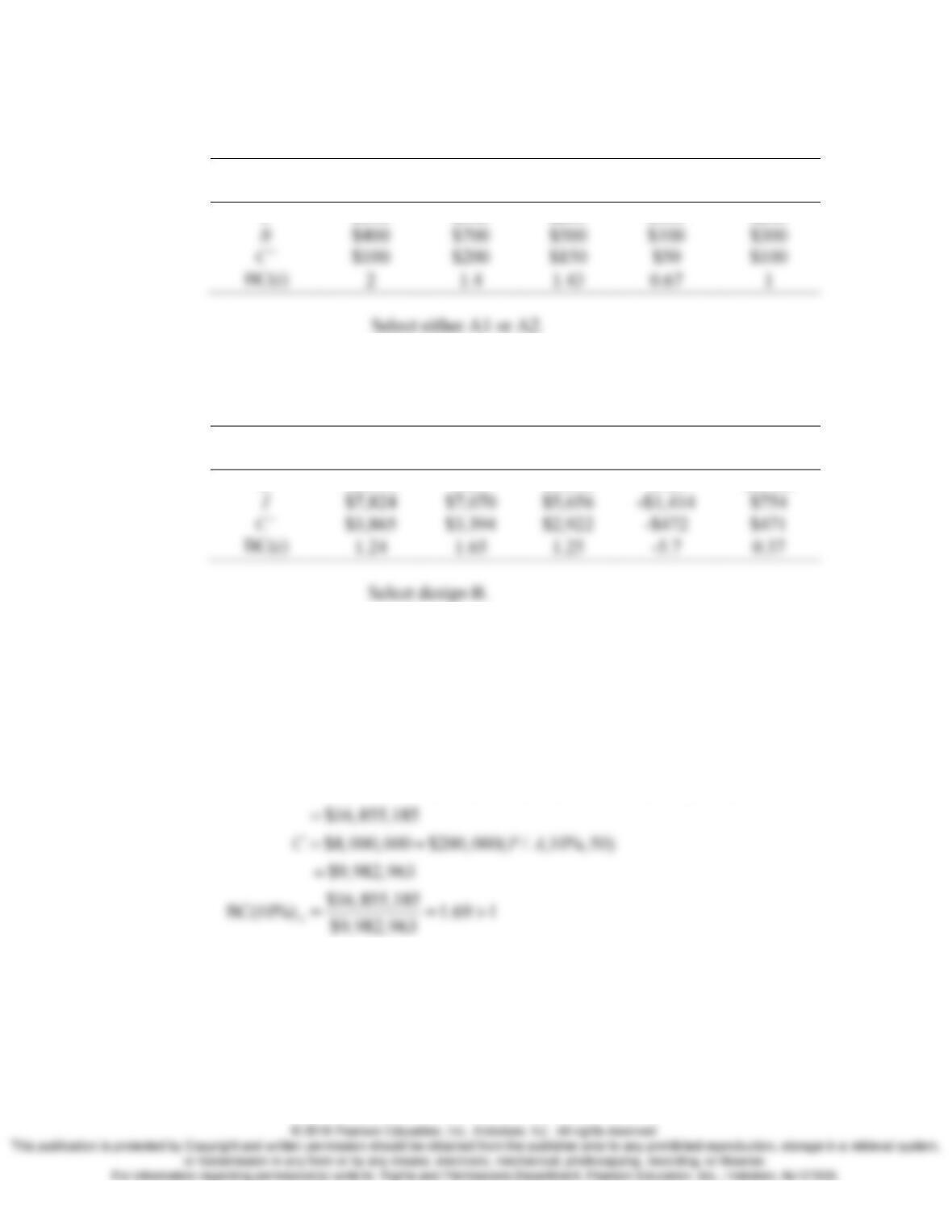
Find the equivalent annual value of each element – I, B, and C’ , as B and C’
are already given on annual basis.
Designs
A
B
C
(b)
(c)
PI(5%)
B-A
=ΔB− ΔC
‘
ΔI
=($40 −$20) −($18 −$8)
($9.32 −$5.83)
16.11 Incremental
BC( )i
analysis:
Present
Worth
Proposals
Incremental
A1
A2
A3
A3–A1
A2–A1
I
$100
$300
$200
$100
$200
16.12 Incremental
BC( )i
analysis:
Present
Worth
Design
Incremental
A
B
C
C-B
A-B
B
$2,440
$880
$1,600
$720
$1,560
I
$754
$3,865
$3,394
$2,922
$471
16.13
(a) The benefit-cost ratio for each alternative:
•Alternative A:
($1,000,000 $250,000 $350,000 $100,000)( / ,10%,50)
BPA
=+++
B
$700
$100
$300
$100
$200
$150
$100
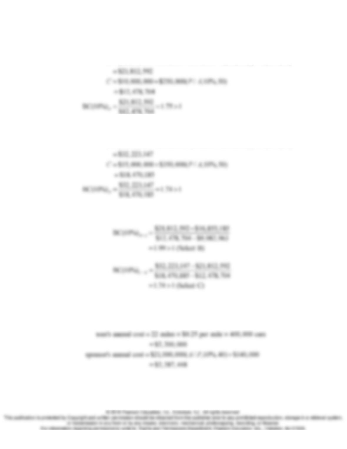
•Alternative B:
($1, 200, 000 $350,000 $450,000 $200,000)( / ,10%,50)
BPA
=+++
•Alternative C:
($1,800,000 $500,000 $600,000 $350,000)( / ,10%,50)
BPA
=+++
(b) Select the best alternative based on
BC( )i
:
16.14
•Option 1 – The “long” route:
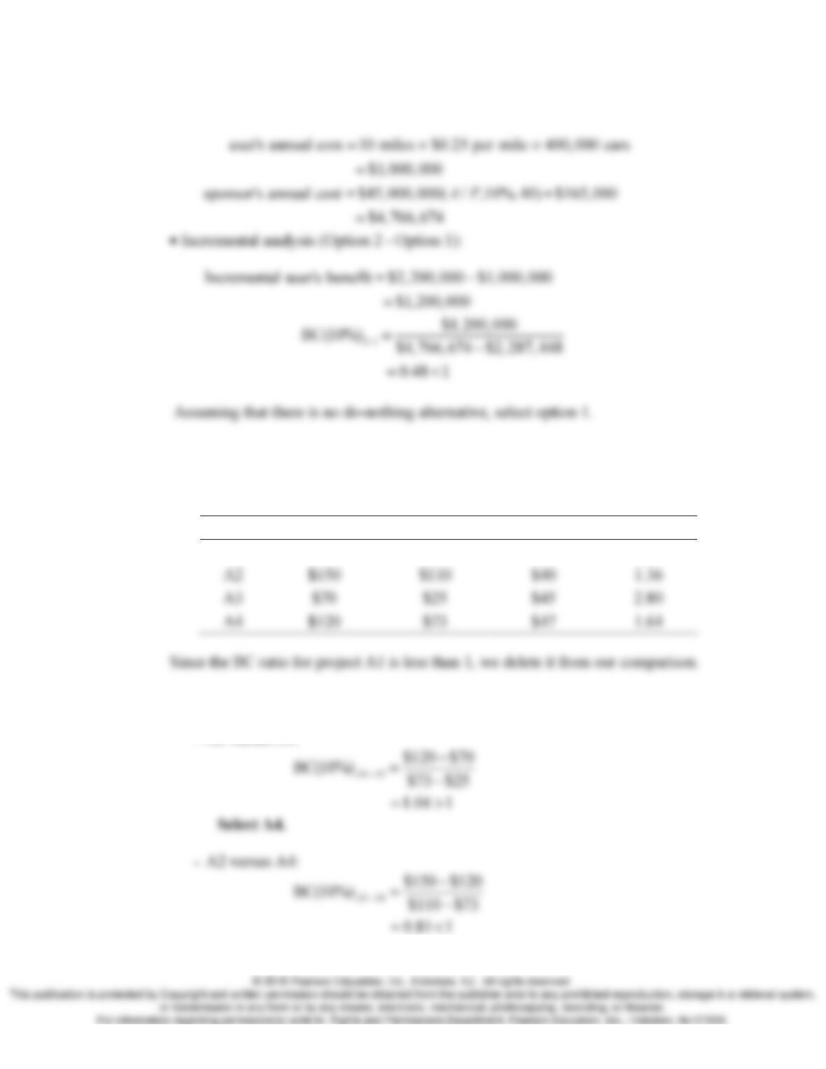
•Option 2 – Shortcut:
16.15
•Multiple alternatives:
Projects
PW of Benefits
PW of Costs
Net PW
B/C ratio
A1
$40
$85
-$45
0.47
A2
$150
1.36
A3
$70
$25
2.80
A4
$120
$73
1.64
•Incremental analysis
– A3 versus A4:
Select A4.
16.16
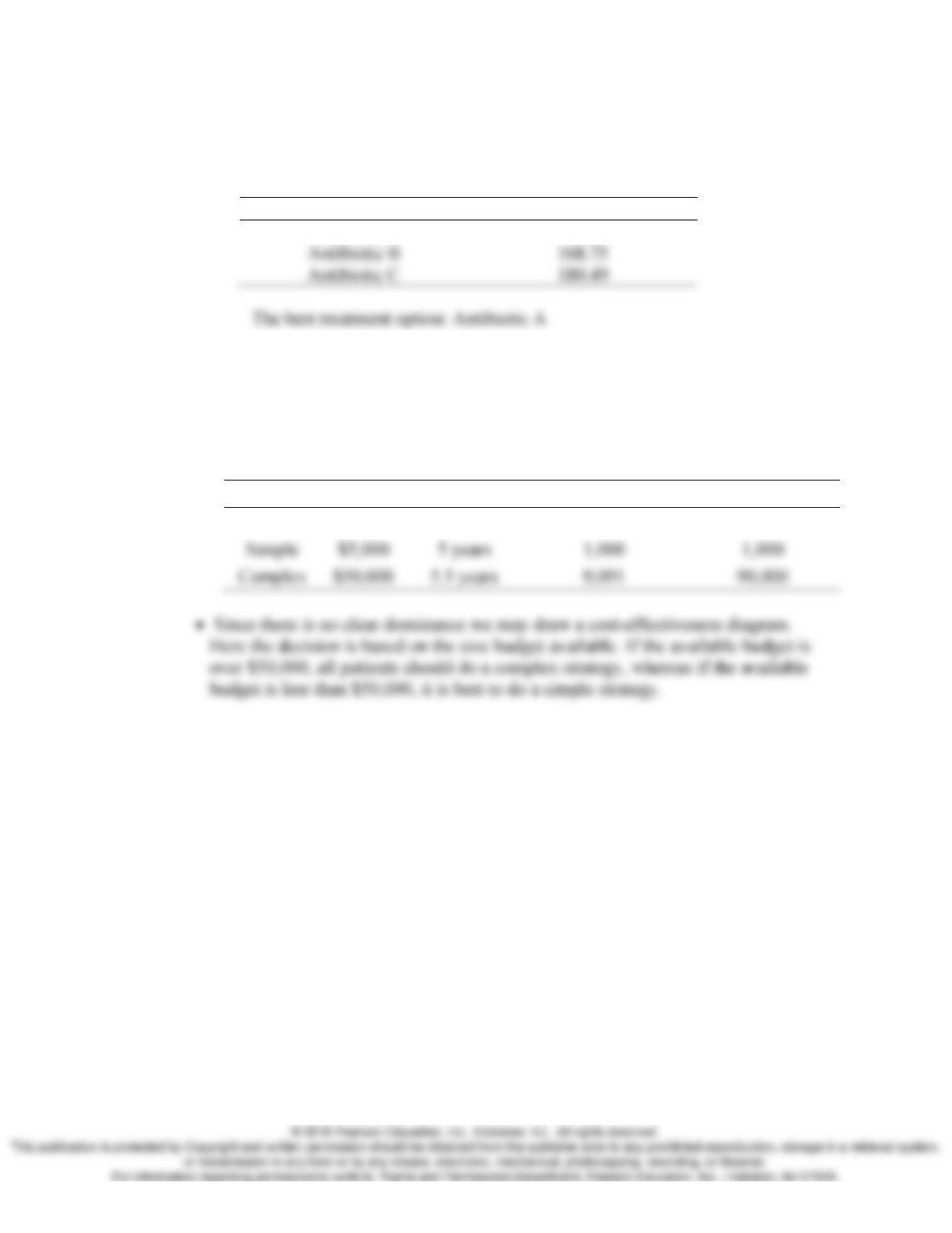
Cost effectiveness of the alternatives
Type of Treatment
Cost Effectiveness
Antibiotic A
160
16.17
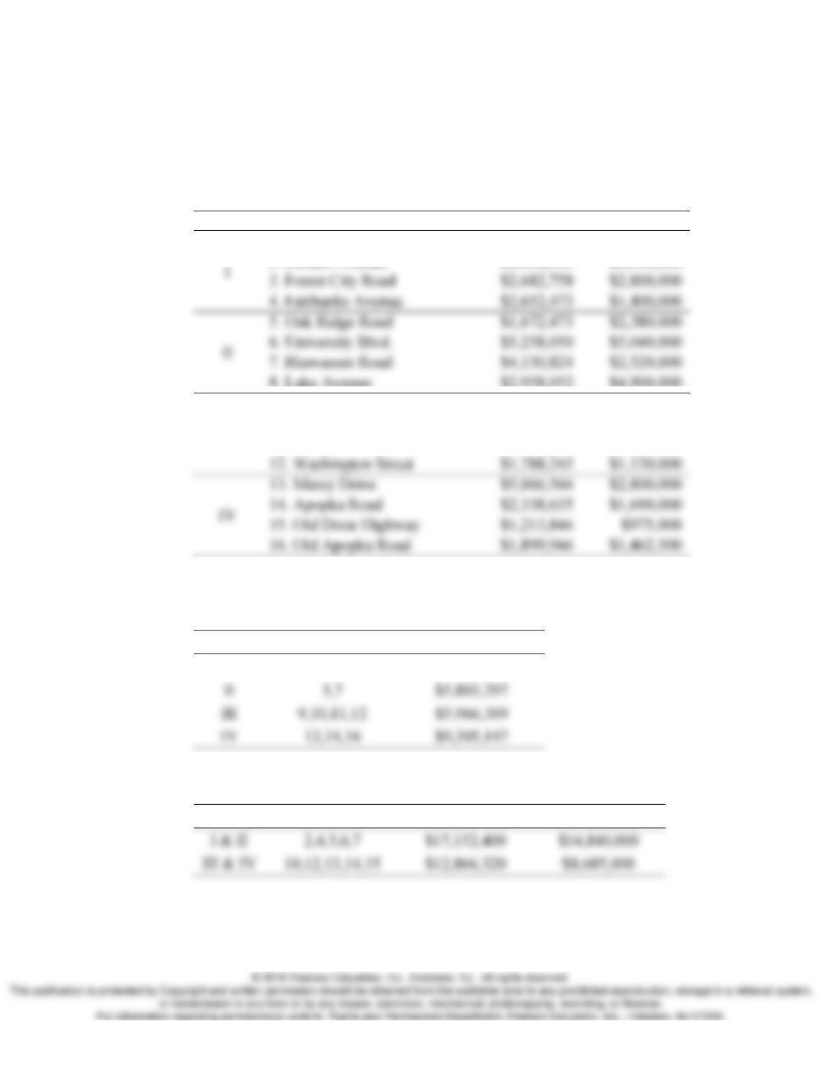
•The summary of three mutually exclusive alternatives CER:
Strategy
Cost
Effectiveness
Cost Effectiveness
Incremental CER
Nothing
$0
0 years
0
0
5 years
Antibiotic C
Short Case Studies
ST 16.1
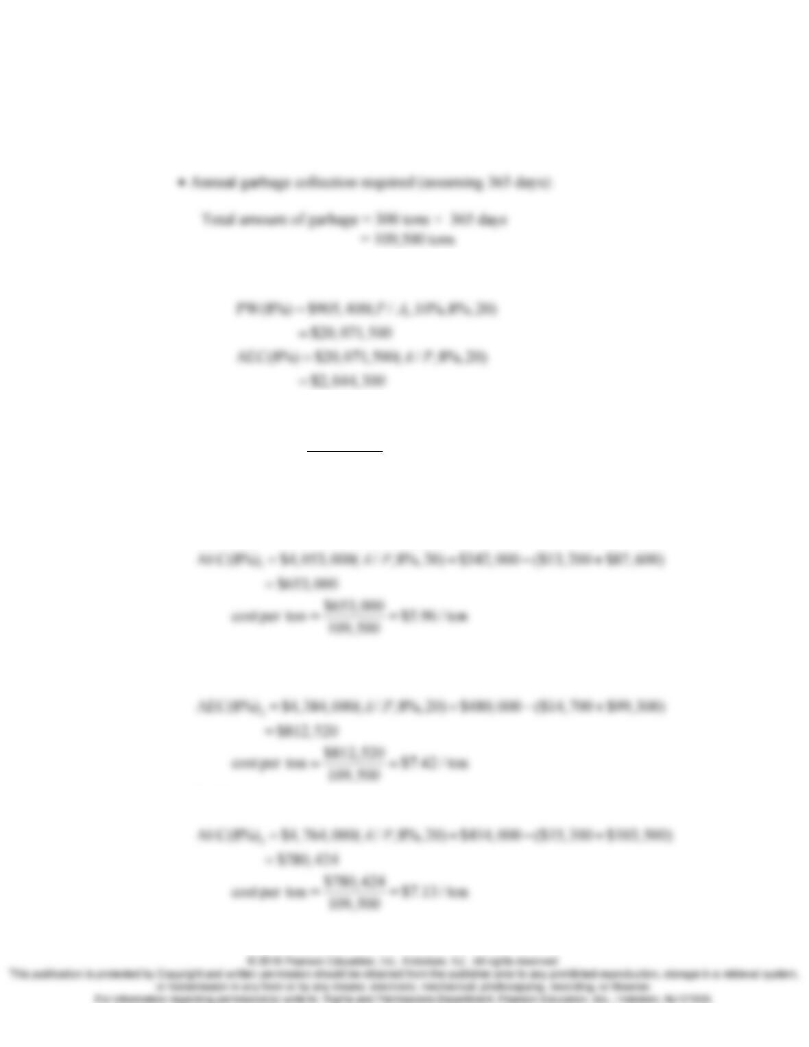
Capital allocation decision, assuming that the government will be able to raise
the required funds at 10% interest:
District
Project
PW(10%)
Investment
1. 27th Street
$1,606,431
$980,000
2. Holden Avenue
$3,438,531
$3,500,000
8. Lake Avenue
$2,958,052
$4,900,000
III
9. Apopka-Ocoee Road
$552,475
$1,365,000
10. Kaley Avenue
$4,459,032
$2,100,000
11. Apopka-Vineland Road
$1,166,557
$1,170,000
12. Washington Street
$1,788,245
$1,120,000
13. Mercy Drive
$5,066,566
$2,800,000
14. Apopka Road
$2,338,635
$1,690,000
15. Old Dixie Highway
$1,213,846
$975,000
16. Old Apopka Road
$1,899,946
$1,462,500
(a) $6 million to each district:
District
Projects
NPW
I
1, 2, 4
$7,697,488
$5,803,297
$5,966,309
(b) $15 million to districts I & II and $9 million to districts III & IV:
District
Projects
NPW
Investment
3. Forest City Road
$2,682,758
$2,800,000
4. Fairbanks Avenue
$2,652,473
$1,400,000
5. Oak Ridge Road
$1,672,473
$2,380,000
6. University Blvd.
$5,258,050
$5,040,000
7. Hiawassee Road
$4,130,824
$2,520,000
ST 16.2 Given
8%i=
,
10%g=
, garbage amount/day = 300 tons
(a) The operating cost of the current system in terms of $/ton of solid waste:
•Equivalent annual operating and maintenance cost:
•Operating cost per ton:
$2,044,300
cost per ton $18.67 / ton
109,500
= =
(b) The economics of each solid-waste disposal alternative in terms of $/ton:
•Site 1:
•Site 2:
•Site 3:
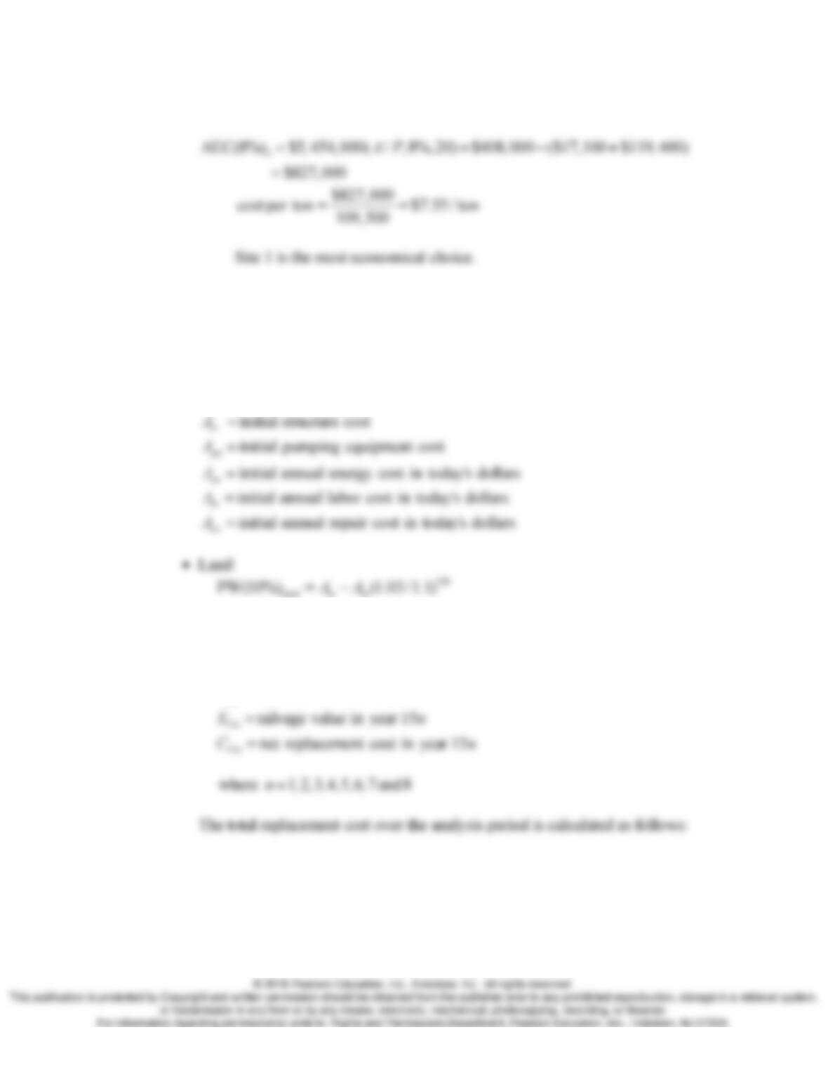
•Site 4:
ST 16.3
(a) Let’s define the following variables to compute the equivalent annual cost.
initial land cost
initial treatment equipment cost
la
eq
A
A
=
=
$0.99963
la
A
=
•Equipment: Let’s define the following additional variables.
15
replacement cost in year 15
n
I n
=
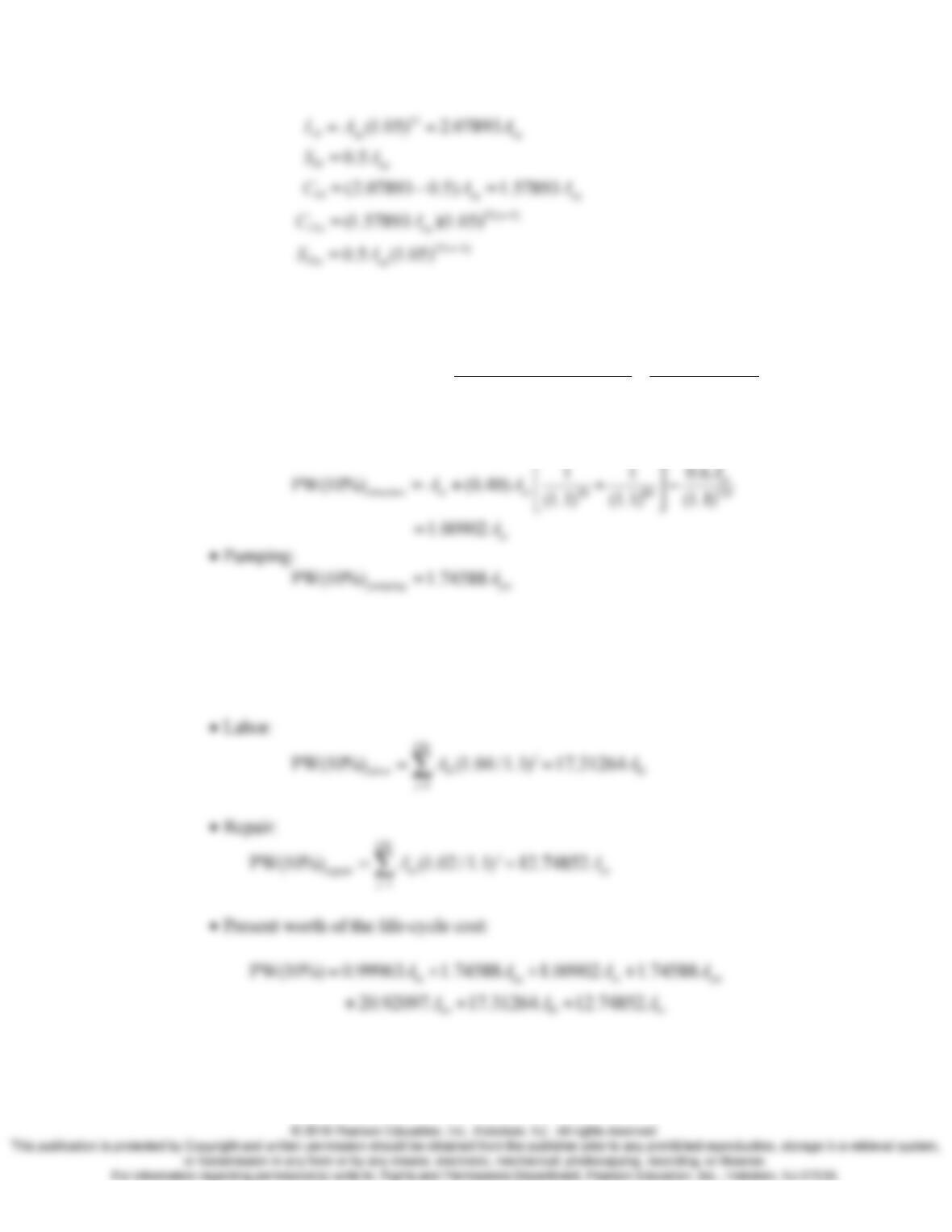
7
15 120
1
15( 1) 105
7
15 120
1
PW(10%)
(1.57893 )(1.05) 0.5 (1.05)
(1.1) (1.1)
1.74588
equipment eq n
n
n
eq eq
eq n
n
eq
ACS
AA
A
A
=
−
=
=+ −
=+ −
=
∑
∑
•Structure:
•Energy:
120
1
PW(10%) (1.05 /1.1) 20.92097
j
energy en en
j
AA
=
==
∑
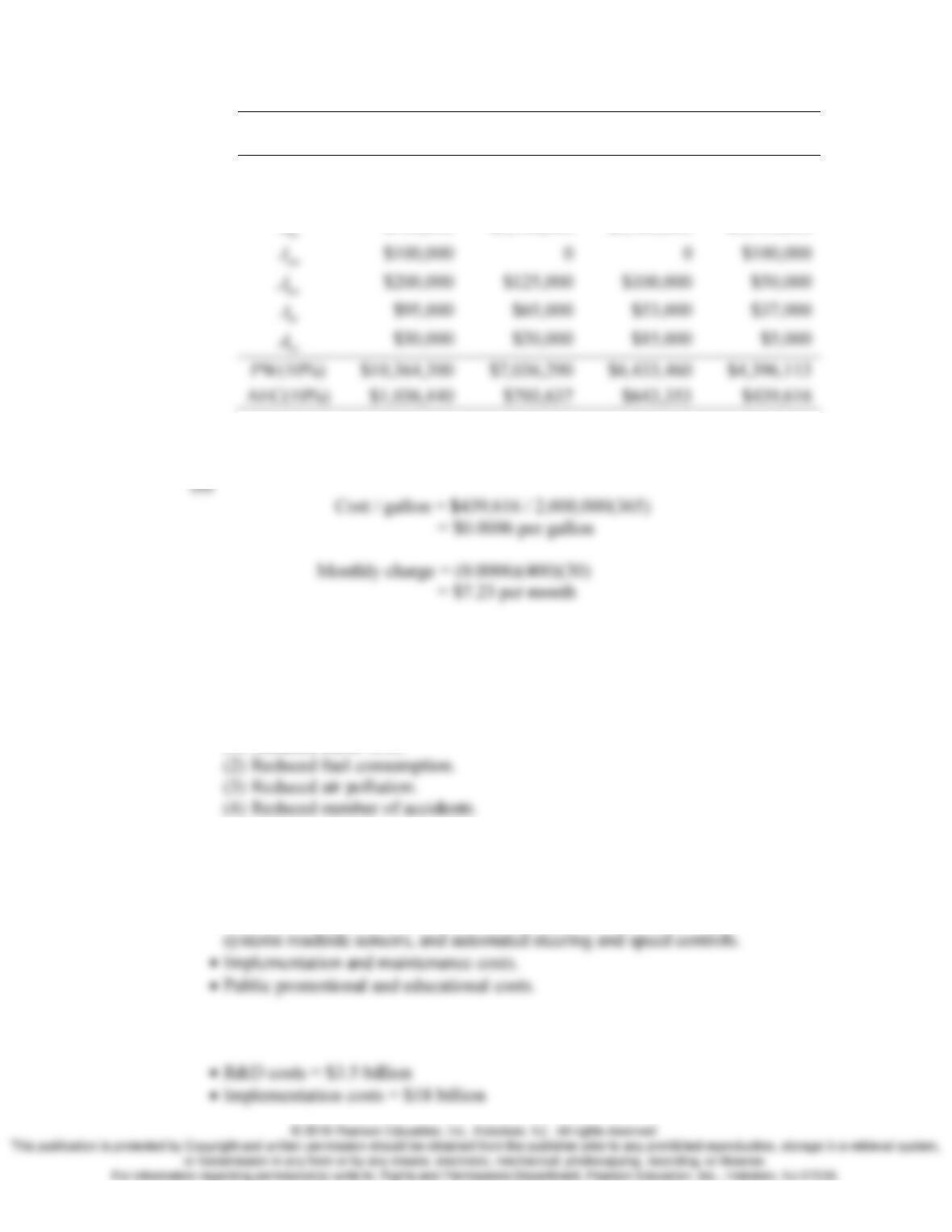
Parameters
Option
2
3
4
5
la
A
$2,400,000
$49,000
$49,000
$400,000
eq
A
$500,000
$500,000
$400,000
$175,000
A
$700,000
$2,100,000
$2,463,000
$1,750,000
Option 5 is the least cost alternative.
ST 16.4
(a) Users benefits and disbenefits:
•Users’ benefits
(1) Reduced travel time.
•Users’ disbenefits: Increased automobile purchase and maintenance costs.
(b) Sponsor’s cost
•Development costs associated with computerized dashboard navigational
(c) On a national level, the sponsor’s costs are estimated to be as follows:
$100,000
$100,000
$200,000
$125,000
$100,000
$65,000
$53,000
$37,000
$20,000
$15,000
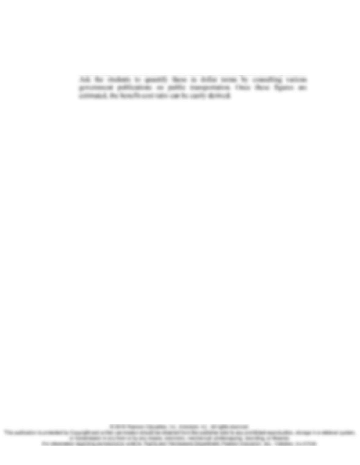
•Maintenance costs = $4 billion per year
Comments: However, the users’ benefits are sketchy, except the level of
reduction possible in the area of travel time, fuel consumption, and air pollution.