
CHAPTER 16
TEACHING NOTES
I spend some time in Section 16.1 trying to distinguish between good and inappropriate uses of
SEMs. Naturally, this is partly determined by my taste, and many applications fall into a gray
area. But students who are going to learn about SEMS should know that just because two (or
Romer’s (1993) inflation and openness example is a nice example of using aggregate cross–
sectional data. Purists may not like the labor supply example, but it has become common to
view labor supply as being a two-tier decision. While there are different ways to model the two
tiers, specifying a standard labor supply function conditional on working is not outside the realm
of reasonable models.
206
SOLUTIONS TO PROBLEMS
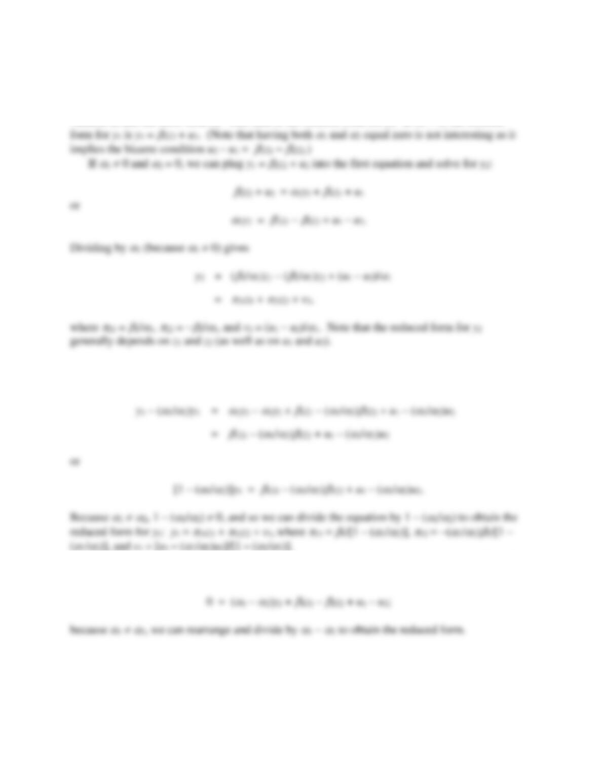
16.1 (i) If
1 = 0 then y1 =
1z1 + u1, and so the right-hand-side depends only on the exogenous
variable z1 and the error term u1. This then is the reduced form for y1. If
1 = 0, the reduced
(ii) If we multiply the second structural equation by (
1/
2) and subtract it from the first
structural equation, we obtain
1/
2)], and v1 = [u1 – (
1/
2)u2]/[1 – (
1/
2)].
A reduced form does exist for y2, as can be seen by subtracting the second equation from the
first:
(iii) In supply and demand examples,
1
2 is very reasonable. If the first equation is the
supply function, we generally expect
1 > 0, and if the second equation is the demand function,
2 < 0. The reduced forms can exist even in cases where the supply function is not upward

207
16.2 Using simple economics, the first equation must be the demand function, as it depends on
16.3 No. In this example, we are interested in estimating the tradeoff between sleeping and
working, controlling for some other factors. OLS is perfectly suited for this, provided we have
16.4 We can easily see that the rank condition for identifying the second equation does not hold:
there are no exogenous variables appearing in the first equation that are not also in the second
16.5 (i) Other things equal, a higher rate of condom usage should reduce the rate of sexually
transmitted diseases (STDs). So
1 < 0.
(ii) If students having sex behave rationally, and condom usage does prevent STDs, then
condom usage should increase as the rate of infection increases.
(iii) If we plug the structural equation for infrate into conuse =
0 +
1infrate + …, we see
(iv) We would have to assume that condis does not appear, in addition to conuse, in the
infrate equation. This seems reasonable, as it is usage that should directly affect STDs, and not

208
16.6 (i) It could be that the decision to unionize certain segments of workers is related to how a
firm treats its employees. While the timing may not be contemporaneous, with the snapshot of a
single cross section we might as well assume that it is.
(ii) One possibility is to collect information on whether workers’ parents belonged to a
16.7 (i) Attendance at women’s basketball may grow in ways that are unrelated to factors that we
can observe and control for. The taste for women’s basketball may increase over time, and this
would be captured by the time trend.
(ii) No. The university sets the price, and it may change price based on expectations of next
year’s attendance; if the university uses factors that we cannot observe, these are necessarily in
(iv) It does make sense to include a measure of men’s basketball ticket prices, as attending a
women’s basketball game is a substitute for attending a men’s game. The coefficient on
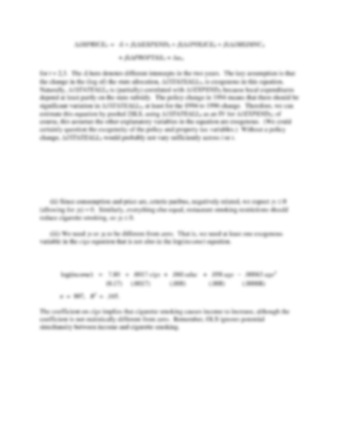
16.8 We must first eliminate the unobserved effect, ai1. If we difference, we have
209
SOLUTIONS TO COMPUTER EXERCISES
C16.1 (i) Assuming the structural equation represents a causal relationship, 100
1 is the
approximate percentage change in income if a person smokes one more cigarette per day.
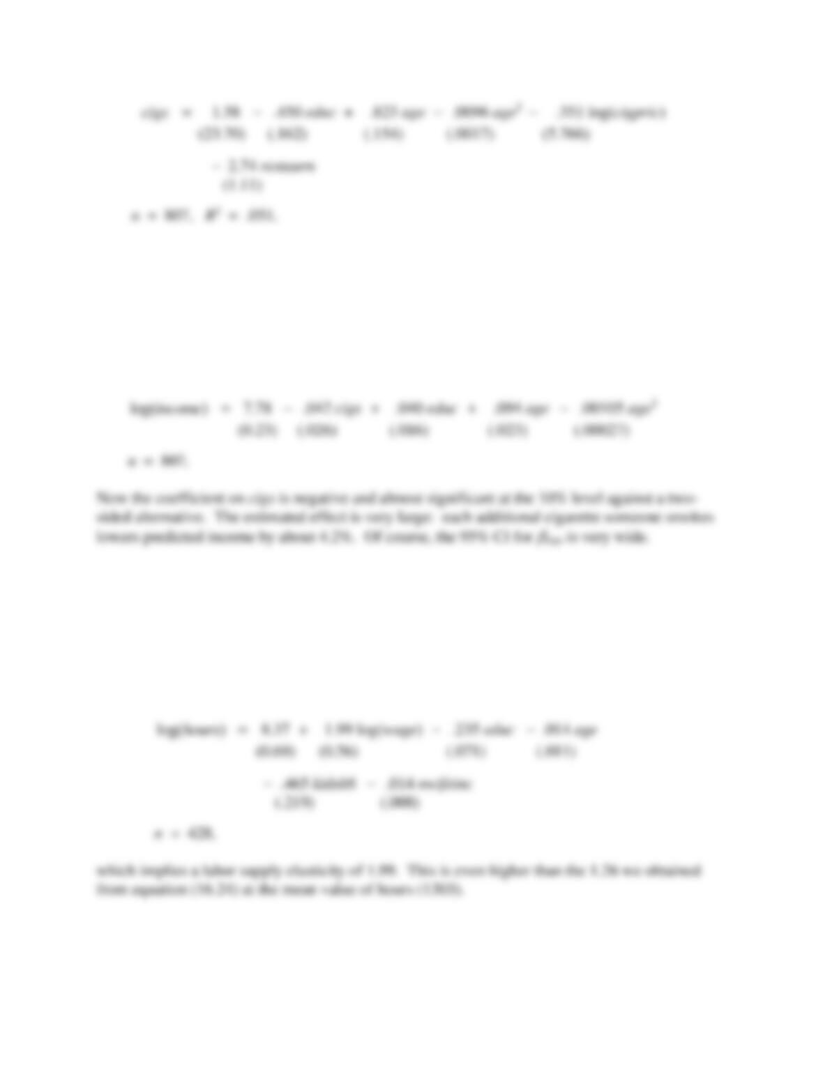
(iv) OLS estimation of the log(income) equation gives
(v) The estimated reduced form for cigs is
210
While log(cigpric) is very insignificant, restaurn had the expected negative sign and a t statistic
of about –2.47. (People living in states with restaurant smoking restrictions smoke almost three
fewer cigarettes, on average, given education and age.) We could drop log(cigpric) from the
analysis but we leave it in. (Incidentally, the F test for joint significance of log(cigpric) and
restaurn yields p-value
.044.)
(vi) Estimating the log(income) equation by 2SLS gives
(vii) Assuming that state level cigarette prices and restaurant smoking restrictions are
exogenous in the income equation is problematical. Incomes are known to vary by region, as do
restaurant smoking restrictions. It could be that in states where income is lower (after controlling
for education and age), restaurant smoking restrictions are less likely to be in place.
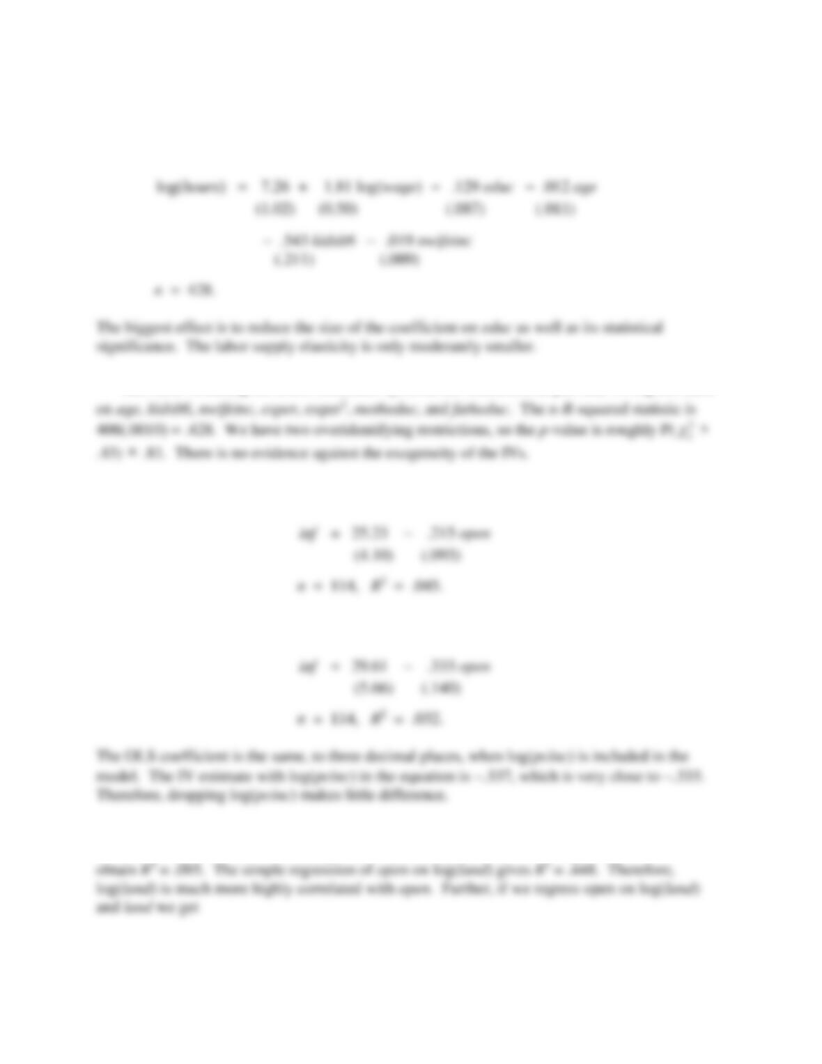
C16.2 (i) We estimate a constant elasticity version of the labor supply equation (naturally, only
for hours > 0), again by 2SLS. We get
211
(ii) Now we estimate the equation by 2SLS but allow log(wage) and educ to both be
endogenous. The full list of instrumental variables is age, kidslt6, nwifeinc, exper, exper2,
motheduc, and fatheduc. The result is
(iii) After obtaining the 2SLS residuals,
ˆ
u
, from the estimation in part (ii), we regress these
C16.3 (i) The OLS estimates are
The IV estimates are
(ii) Subject to the requirement that an IV be exogenous, we want an IV that is as highly
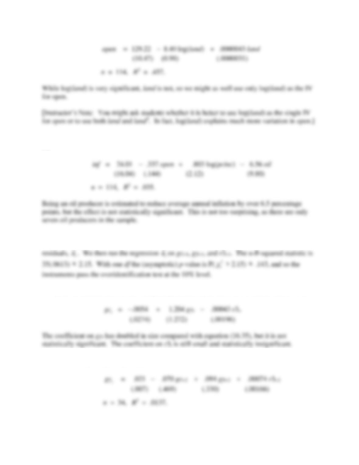
correlated as possible with the endogenous explanatory variable. If we regress open on land we
212
(iii) When we add oil to the original model, and assume oil is exogenous, the IV estimates
are
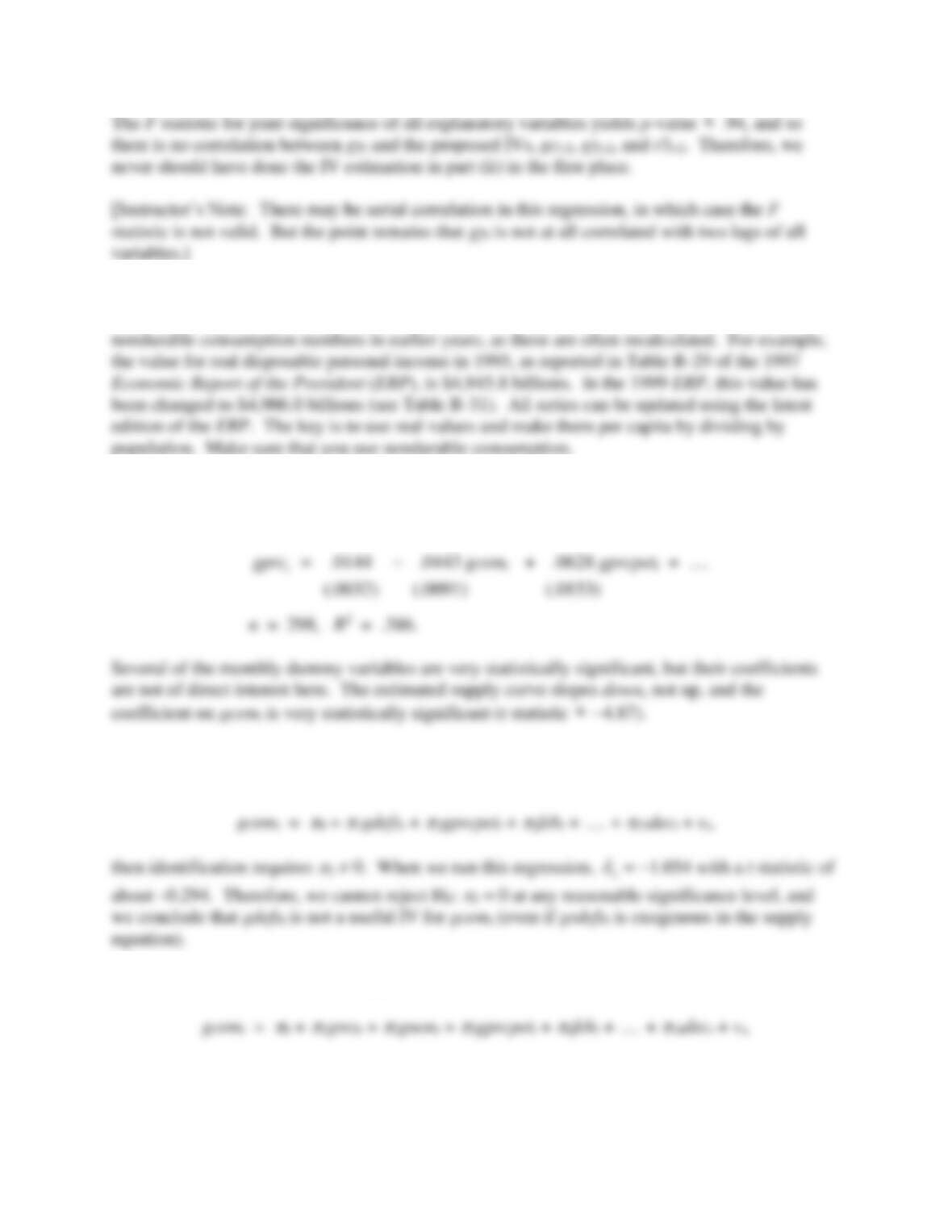
C16.4 (i) The usual form of the test assumes no serial correlation under H0, and this appears to
be the case. We also assume homoskedasticity. After estimating (16.35), we obtain the 2SLS
(ii) If we estimate (16.35) but with gct-2, gyt-2, and r3t-2 as the IVs, we obtain, with n = 34,
(iii) If we regress gyt on gct-2, gyt-2, and r3t-2 we obtain
213
C16.5 This is an open-ended question without a single answer. Even if we settle on extending
the data through a particular year, we might want to change the disposable income and
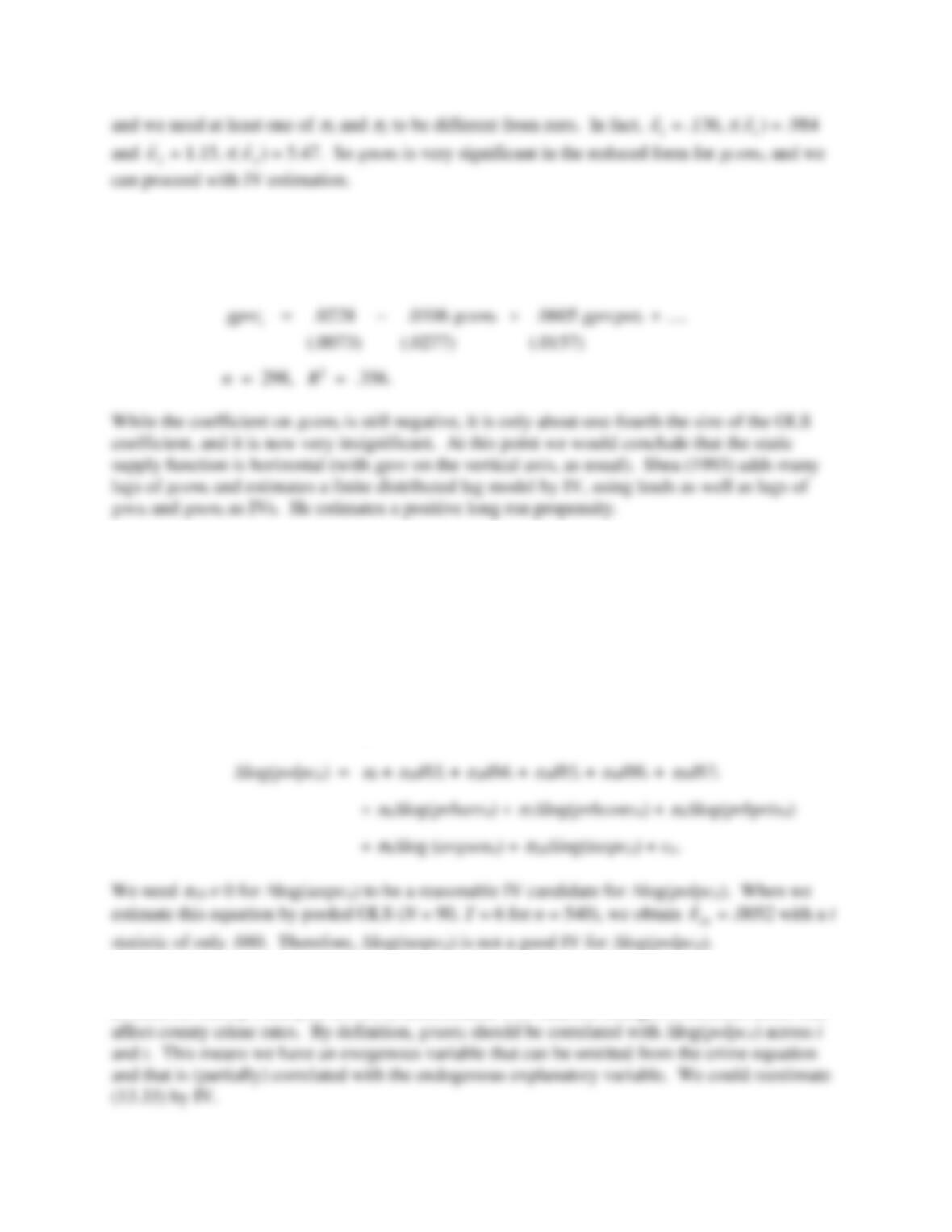
C16.6 (i) If we estimate the inverse supply function by OLS we obtain (with the coefficients on
the monthly dummies suppressed)
(ii) We need gdefst to have a nonzero coefficient in the reduced form for gcemt. More
precisely, if we write
(iii) Now the reduced form for gcem is
214
(iv) We use both grest and gnont as IVs for gcemt and apply 2SLS, even though the former is
not significant in the RF. The estimated labor supply function (with seasonal dummy
coefficients suppressed) is now
C16.7 (i) If county administrators can predict when crime rates will increase, they may hire more
police to counteract crime. This would explain the estimated positive relationship between
log(crmrte) and log(polpc) in equation (13.33).
(ii) This may be reasonable, although tax collections depend in part on income and sales
taxes, and revenues from these depend on the state of the economy, which can also influence
crime rates.
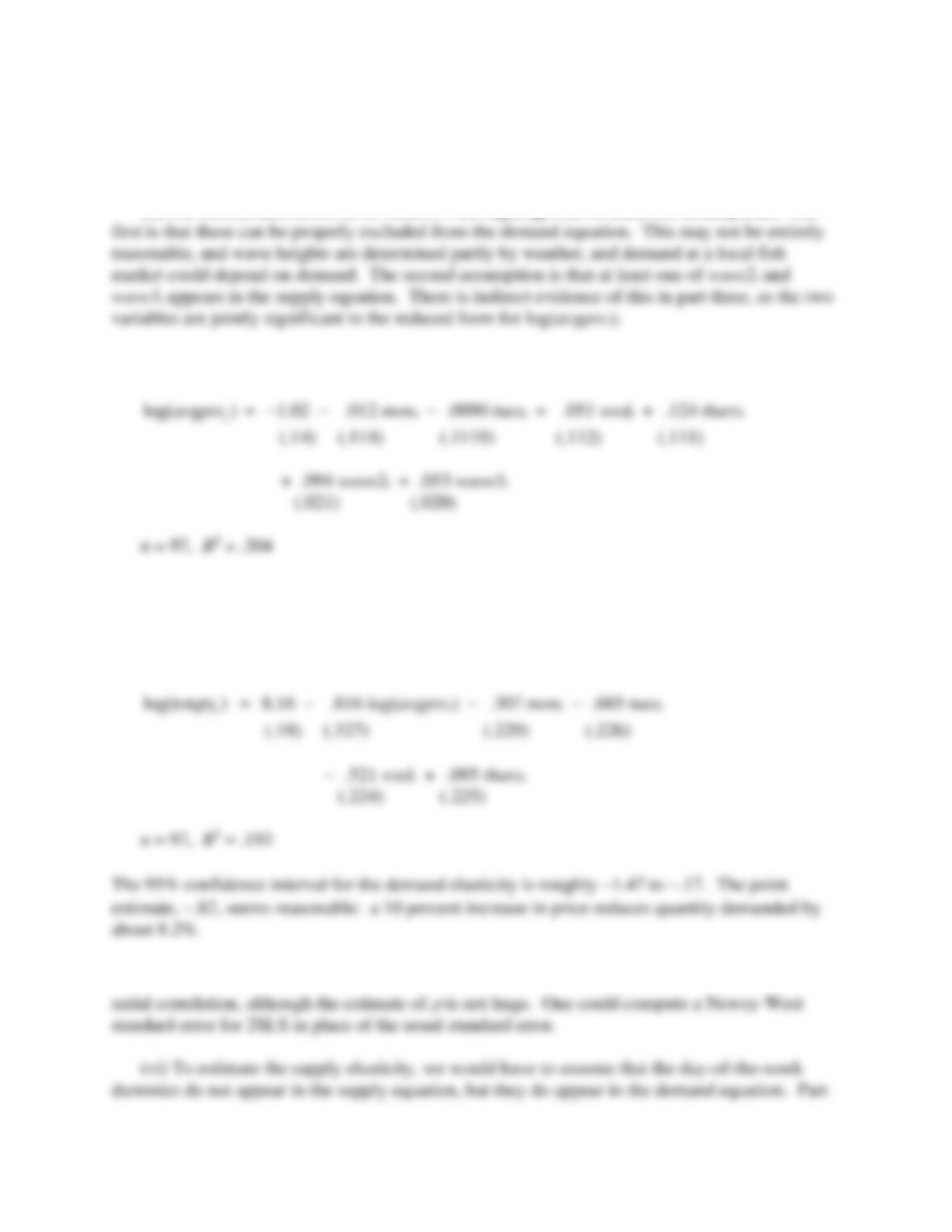
(iii) The reduced form for log(polpcit), for each i and t, is
(iv) If the grants were awarded randomly, then the grant amounts, say grantit for the dollar
amount for county i and year t, will be uncorrelated with uit, the changes in unobservables that
215
C16.8 (i) To estimate the demand equations, we need at least one exogenous variable that
appears in the supply equation.
(ii) For wave2t and wave3t to be valid IVs for log(avgprct), we need two assumptions. The
(iii) The OLS estimates of the reduced form are
The variables wave2t and wave3t are jointly very significant: F = 19.1, p-value = zero to four
decimal places.
(iv) The 2SLS estimates of the demand function are
(v) The coefficient on
,1
ˆit
u−
is about .294 (se = .103), so there is strong evidence of positive
216
(iii) provides evidence that there are day-of-the-week effects in the demand function. But we
cannot know about the supply function.
(vii) Unfortunately, in the estimation of the reduced form for log(avgprct) in part (iii), the
C16.9 (i) The demand function should be downward sloping, so
1
< 0: as price increases,
quantity demanded for air travel decreases.
(ii) The estimated price elasticity is −.391 (t statistic = −5.82).
(iii) We must assume that passenger demand depends only on air fare, so that, once price is
The coefficient on concen shows a pretty strong link between concentration and fare. If concen
increases by .10 (10 percentage points), fare is estimated to increase by almost 4%. The t
statistic is about 6.3.
(v) Using concen as an IV for log(fare) [and where the distance variables act as their own
217
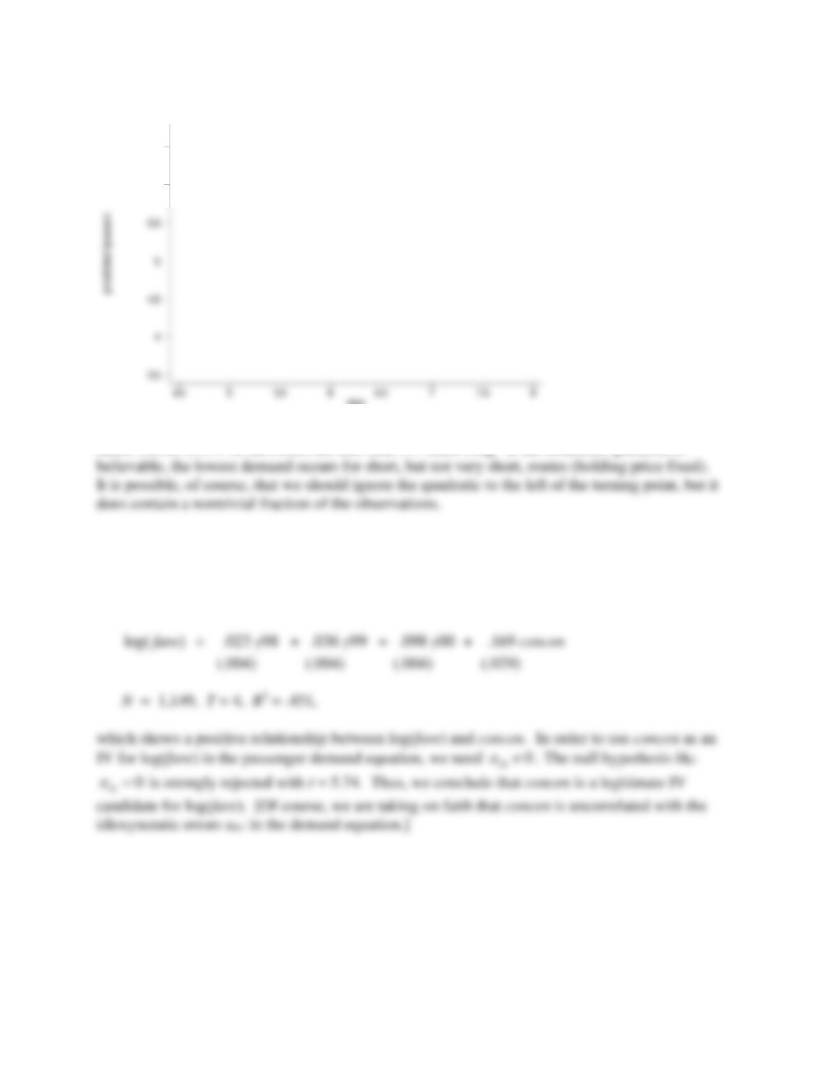
The minimum is at about ldist = 2.176/.187 5.82, which, in terms of distance, is about 337
miles. About 11.3% of the routes are less than 337 miles long. If the estimated quadratic is
C16.10 (i) The FE estimate of the elasticity is −1.155 with standard error .023, and so the
estimate is economically large and very statistically significant.
(ii) The FE estimates of the reduced form are
(iii) Use fixed effects IV, the estimated elasticity is −.302, which is much smaller in
magnitude than the usual FE estimate. Plus, the t statistic for the elasticity is now only −1.09, so
the estimated elasticity is not statistically different from zero.
ldist
6
6.5

218
C16.11 (i) Logically, sfood has to be between zero and one. In this sample, it ranges from a low
of about .057 to a high of .789. It is not surprising to see no zeros; presumably everyone has to
spend something on food (except maybe a completely self-sufficient farmer who does not put a
price on his or her own food).
(ii) The coefficient on ltotexpend is −.146 with a robust standard error of .0062. If
(iii) The reduced form equation is
(iv) When (16.43) is estimated by IV, using lincome as an instrument for ltotexpend, the
(v) When we obtain the reduced form residuals, say
2
ˆ
v
2
ˆ
v
, from part (iii) and add them to
(vi) The OLS estimate of the ltotexpend coefficient is .028 (robust t = 6.66) while the IV