Basic Econometrics, Gujarati and Porter
182
CHAPTER 16:
PANEL DATA REGRESSION MODELS
16.1 In cross-sectional data we gather information about several
microunits at the same point in time. It is generally assumed that
16.2 In a fixed effects model (FEM) we allow each microunit to be
16.3 In the error components model (ECM), unlike FEM, we assume
that the intercept of a microunit is a random drawing with certain
16.4 They are all synonymous.
16.5 The answer is provided in Sec. 16.1. Briefly, by combining both
16.6 The new error term will be:
with the assumptions that
Basic Econometrics, Gujarati and Porter
183
2 2 2 2
var( )
it u
w
ε ν
σ σ σ σ
= = + +
u
it jt
ε ν
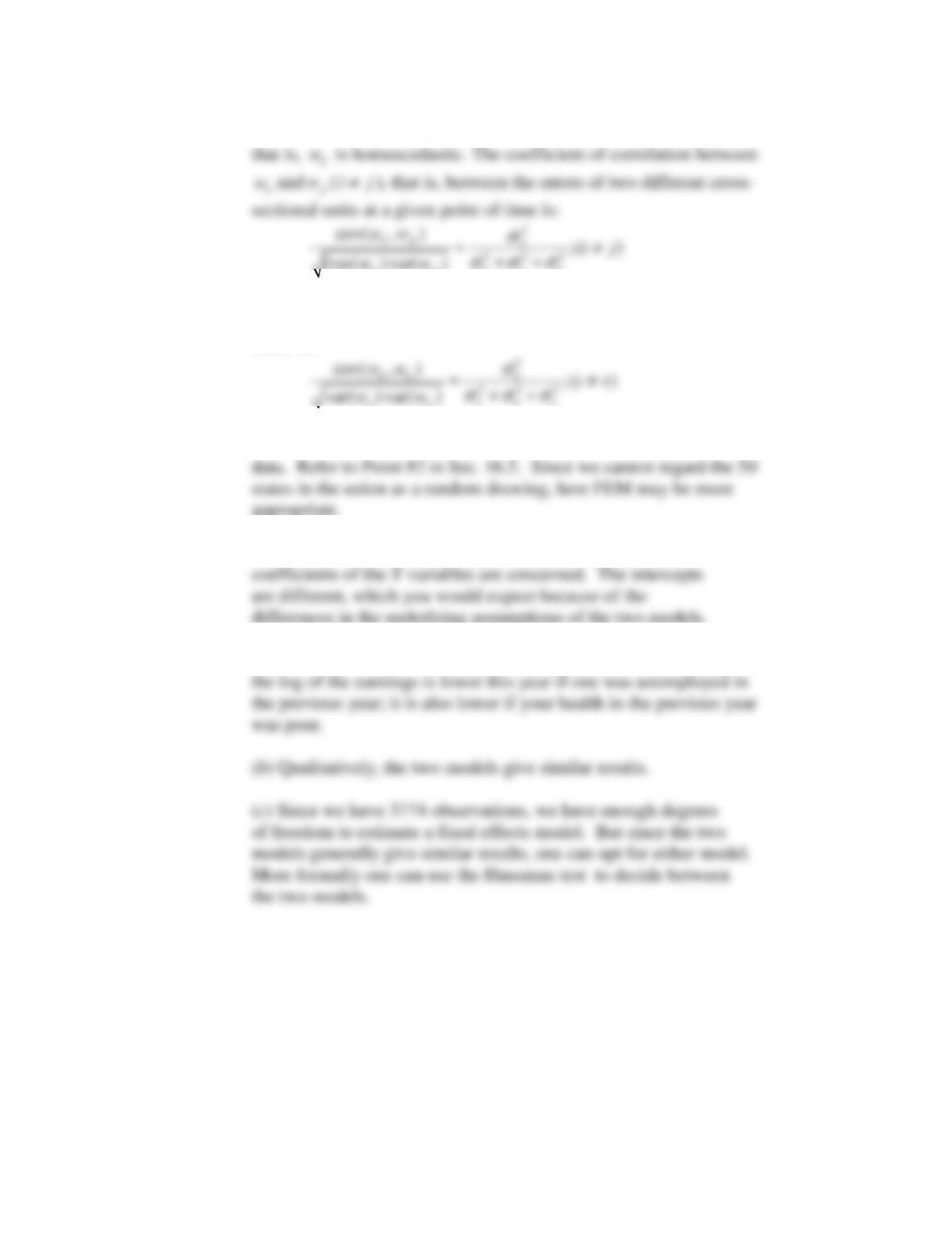
And the coefficient of correlation between
and ( )
it jt
w w t s
≠
, that is,
between the errors of a given cross-sectional unit at two different
times is,
16.7
Here we have N = 50 cross-sectional units and T = 2 time series
16.8
The results are not substantially different insofar as the
16.9
(a) On the whole, the results make economic sense. For example,
Empirical Exercises
16.10
Results for the log-linear model are as follows:
Basic Econometrics, Gujarati and Porter
184
Dependent Variable: LN_C
Method: Least Squares
Sample: 1 90
Included observations: 90
Variable Coefficient Std. Error t-Statistic Prob.
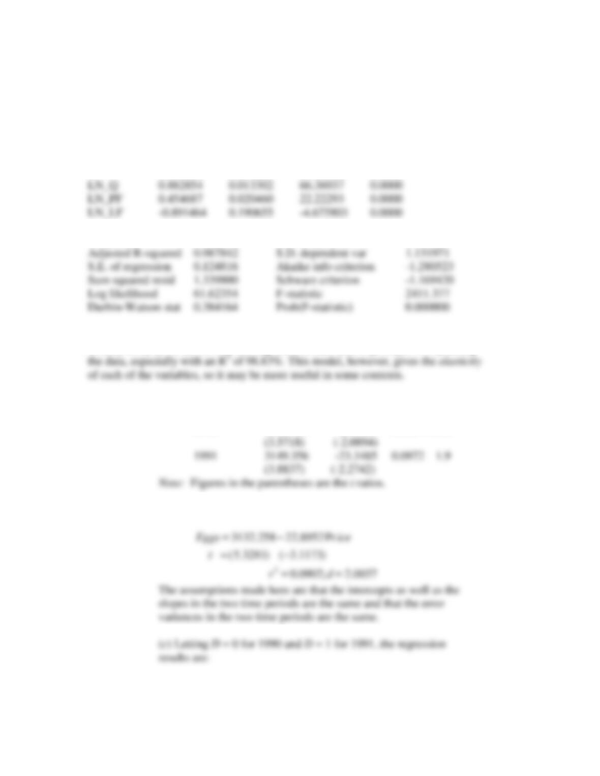
C 8.075649 0.334203 24.16392 0.0000
R-squared 0.988252 Mean dependent var 13.36561
Keeping in mind that we cannot compare these results to those in Table 16.2
directly (why?), we do see that this log-linear model does a good job of explaining
16.11
(a) Year Intercept slope R
2
d
1990 3118.484 -22.4984 0.0834 1.98
(b) The pooled regression results are as follows:
Basic Econometrics, Gujarati and Porter
185
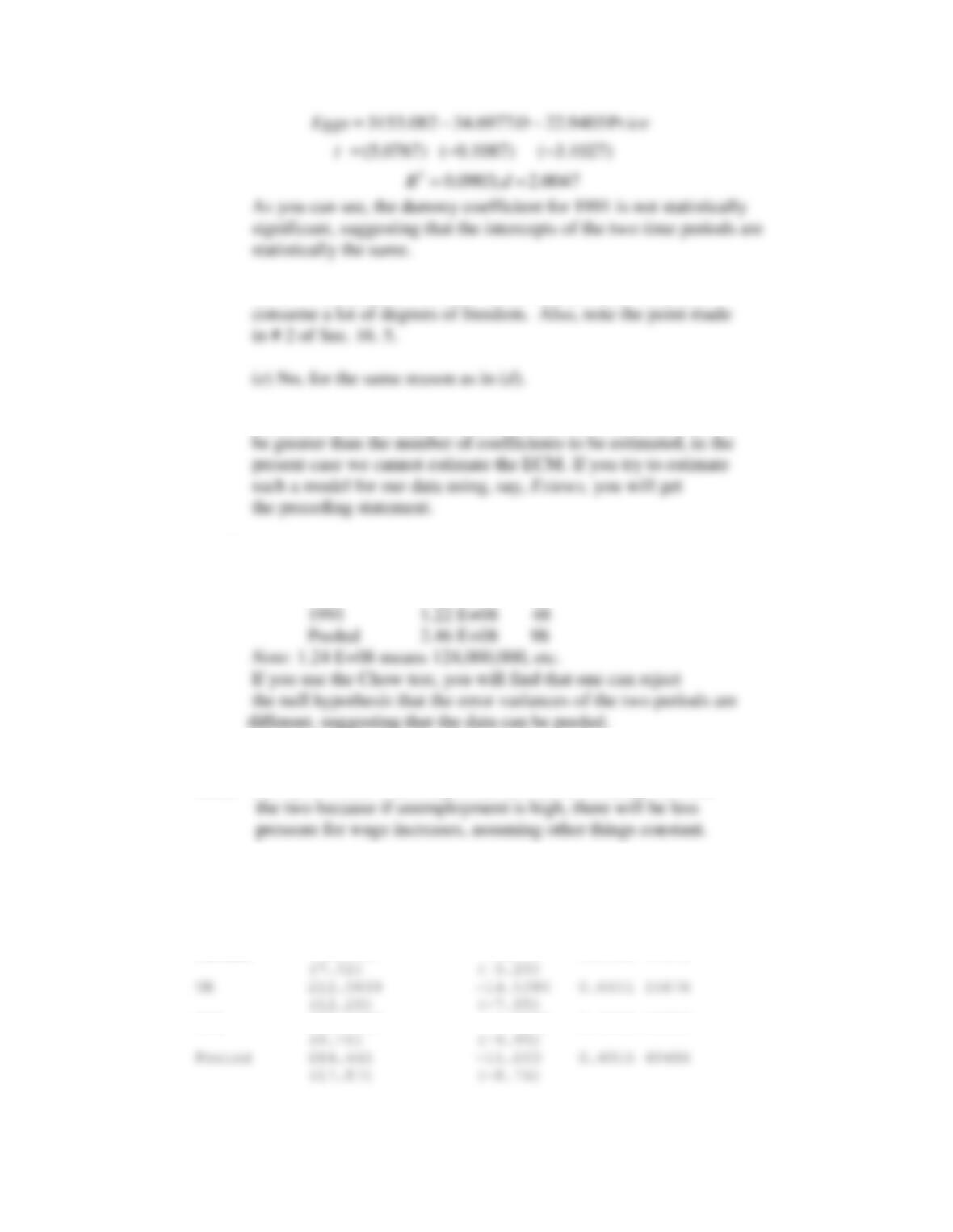
(d) If we do that, we will have to use 49 dummies. This will
(f) Since the ECM requires the number of cross-sectional units to
16.12
Here are the necessary data:
Year RSS df
1990
1.24 E+08 48
16.13
(a) A priori one would expect an inverse relationship between
(b) & (c) In tabular form, the results are as follows (t ratios in
parentheses):
Country Intercept Slope R
2
RSS
Canada 155.9507 -7.8523 0.2908 11878
USA 202.1487 -15.5595 0.4415 16895
Basic Econometrics, Gujarati and Porter
186
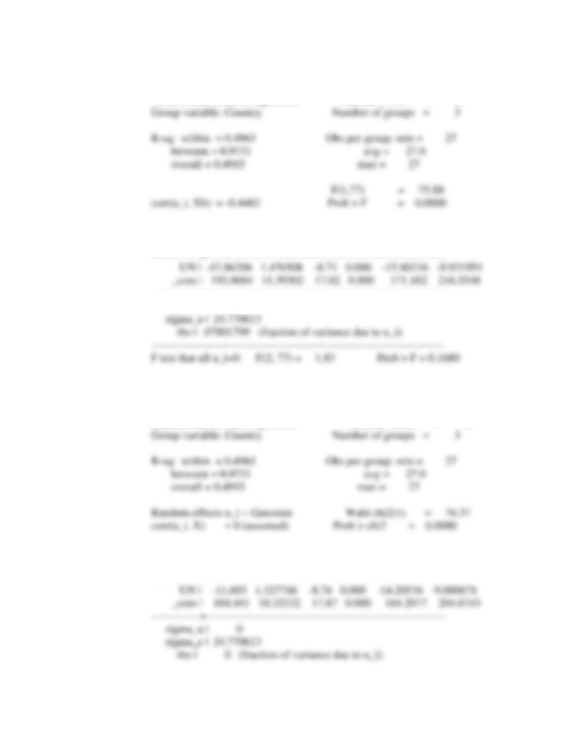
(d) The results here and in (e) below are obtained from Stata.
Fixed-effects (within) regression Number of obs = 81
————————————–—————-——————–—-
comp | Coef. Std. Err. t P>|t| [95% Conf. Interval]
————-+—————————————-——————–—-
sigma_u | 7.2056457
(e) From Stata:
Random-effects GLS regression Number of obs = 81
————————————–—————-——————–—-
comp | Coef. Std. Err. z P>|z| [95% Conf. Interval]
————-+—————————————-——————–—-
Basic Econometrics, Gujarati and Porter
187
————————————–—————-——————–—-
16.14
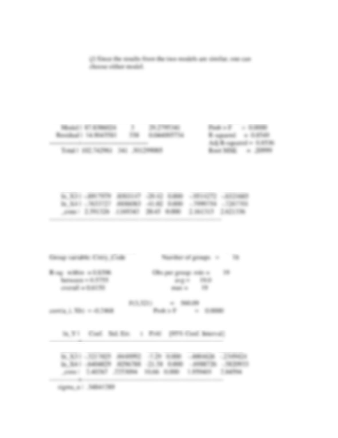
(a) Stata results for the pooled model are:
regress ln_Y ln_X2 ln_X3 ln_X4
Source | SS df MS Number of obs = 342
————-+—————————— F( 3, 338) = 664.00
————————————–—————-——————–—-
ln_Y | Coef. Std. Err. t P>|t| [95% Conf. Interval]
————-+—————————————-——————–—-
ln_X2 | .8899616 .0358058 24.86 0.000 .8195313 .9603919
(b) Fixed effects results from Stata are:
Fixed-effects (within) regression Number of obs = 342
————————————–—————-——————–—-
————-+—————————————-——————–—-
ln_X2 | .6622498 .073386 9.02 0.000 .5178715 .8066282
Basic Econometrics, Gujarati and Porter
188
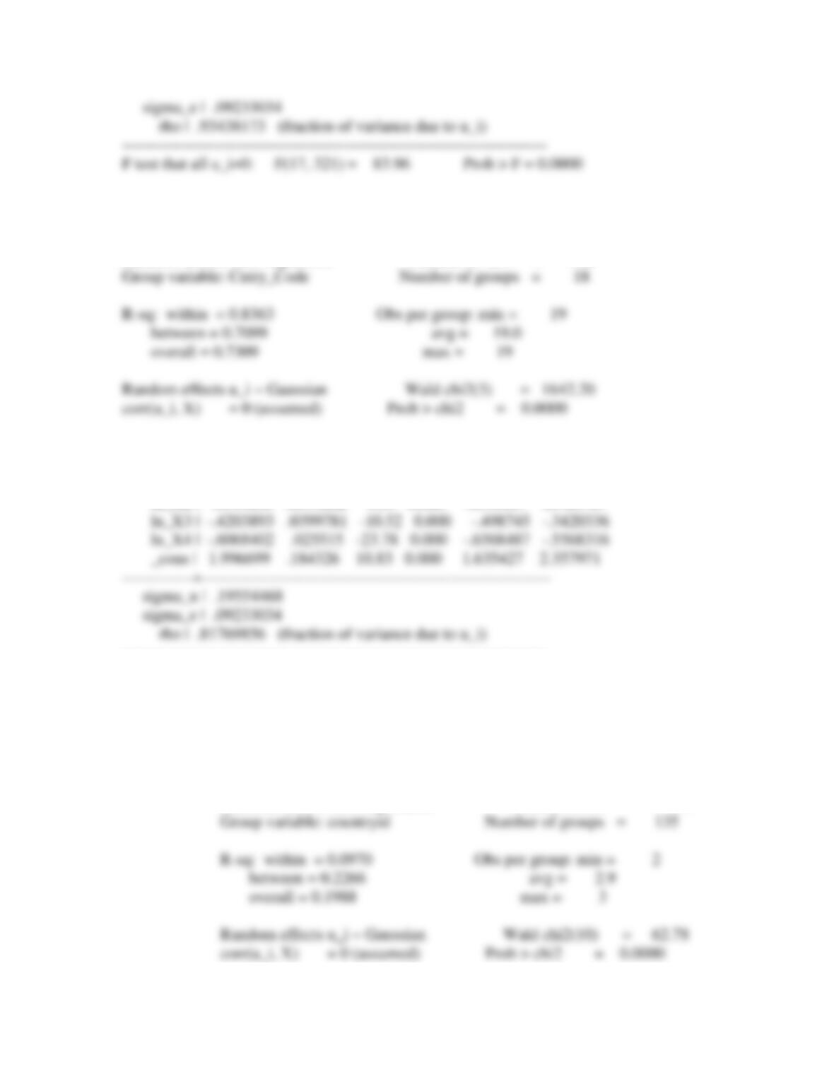
(c) Random effects model from Stata is:
Random-effects GLS regression Number of obs = 342
————————————–—————-——————–—-
ln_Y | Coef. Std. Err. z P>|z| [95% Conf. Interval]
————-+—————————————-——————–—-
ln_X2 | .5549858 .0591282 9.39 0.000 .4390967 .6708749
————————————–—————-——————–—-
(d) Again it seems that both the fixed and random effects models have similar results.
The reader can apply the Hausman test to validate this and choose the most appropriate
one.
16.15
The following are the Stata results for a random effects model:
Random-effects GLS regression Number of obs = 395
Basic Econometrics, Gujarati and Porter
189
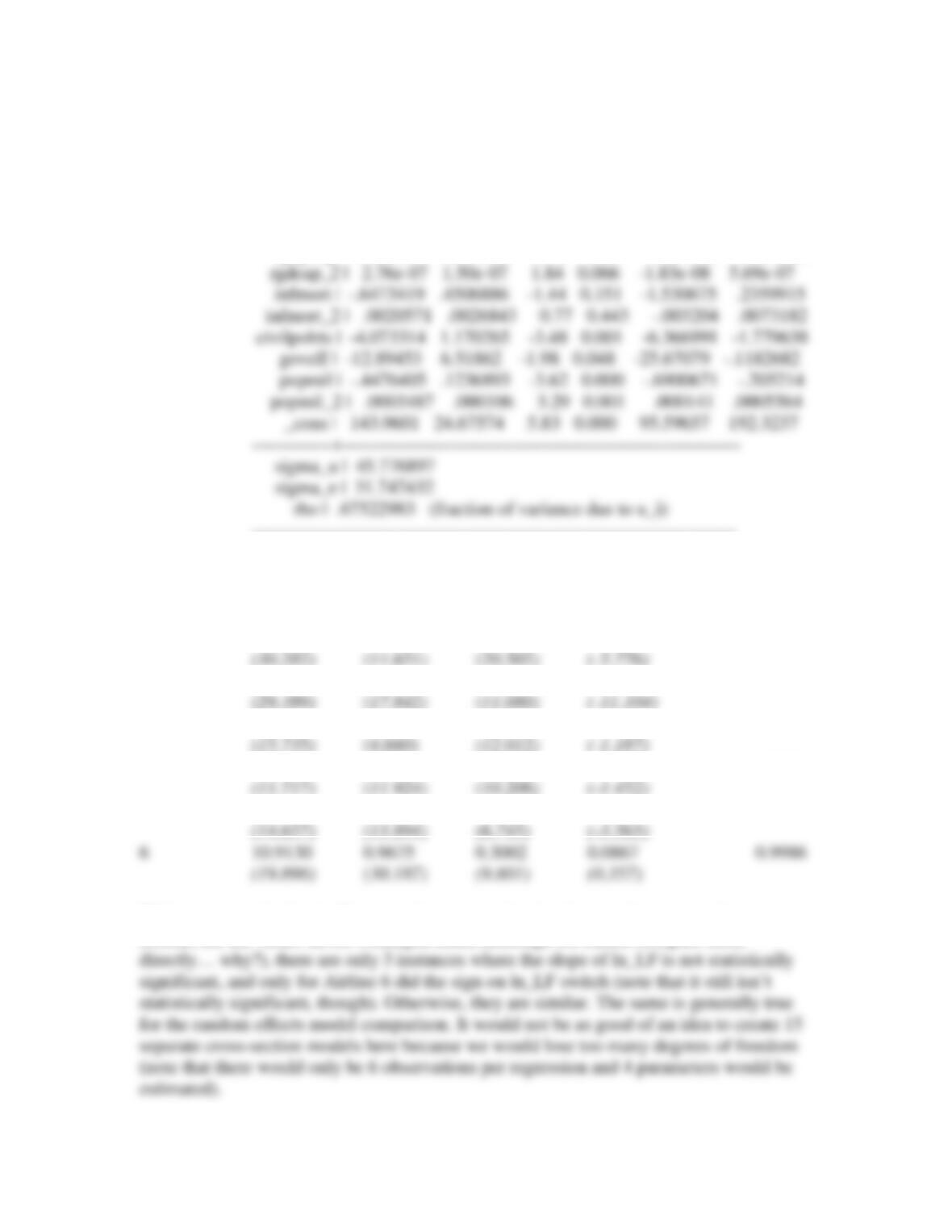
————————————–—————-——————–—-
aidcap | Coef. Std. Err. z P>|z| [95% Conf. Interval]
————-+—————————————-——————–—-
y2 | -20.97589 4.034306 -5.20 0.000 -28.88299 -13.0688
y3 | -17.74298 4.233206 -4.19 0.000 -26.03991 -9.446051
rgdpcap | -.0068197 .0035383 -1.93 0.054 -.0137546 .0001152
————————————–—————-——————–—-
16.16
For each airline: (values in parentheses are t statistics)
Airline Intercept Slope ln_Q Slope ln_PF Slope ln_LF R
2
1 8.5592 1.1664 0.3917 -1.4614 0.998
2 9.5408 1.4649 0.3104 -1.5216 0.9988
3 8.0011 0.7196 0.4534 -0.4241 0.9940
4 8.5738 0.9371 0.4590 -0.3765 0.9951
5 10.6531 1.0618 0.2959 -0.6132 0.9981
With respect to the fixed effects results presented in the chapter, the outputs above are
similar; the R2 values haven’t changed much (although we cannot compare them