Table 16.1 Additional Funds Needed (AFN) Model (Millions of Dollars) 12/12/2018
Part I. 2019 Data from Chapter 3, Tables 3.1 and 3.2
A0* = Assets at 12/31/19. All assets were needed for 2019 sales $2,000
S0 = 2019 Sales $3,000
Part II. Data Used in the AFN Equation: 2019 Ratios Held Constant
Base Case:
2019 Data
0.6667
0.0488
0.4101
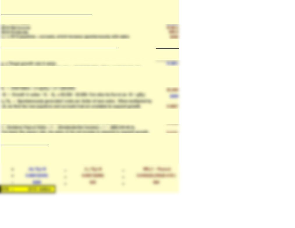
Part III. The AFN Equation
AFN = – –
Required increase
in assets
Spontaneous
increase in payables
and accruals
Funds obtained as new
retained earnings. Based
on 2020 sales
AFN = Additional Funds Needed to buy assets needed to support growth. AFN is
in addition to funds raised internally, i.e., AFN represents required external funds.
A0*/S0 = Assets required per $1 of sales = $2,000/$3,000. When multiplied by the
increase in sales shows the required new assets for the coming year. Also called the
capital intensity ratio . The higher this ratio, the more new assets the firm will need to
support a given amount of growth.
M = Profit margin on sales = 2019 net income/S0 = $146.3/$3,000. Multiply by S1 (not
S0) to find the net income available in 2020 for dividends or growth.
The lower the payout rate, the more of the net income is retained to support growth.
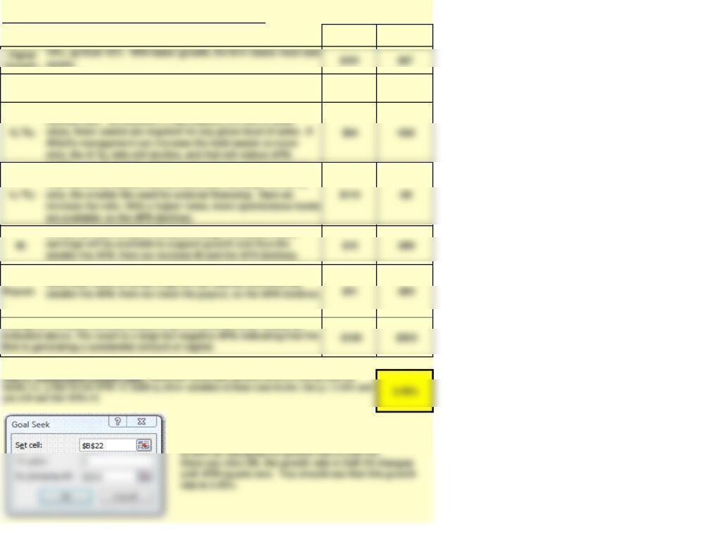
Part IV. Sensitivity Analysis: AFN with Changed Input Values
New
Change:
New – Old
Growth:
Lower
Growth:
$27 -$87
The sustainable growth rate is found using
Excel’s Goal Seek. AFN (calculated in Cell B22) is set
to zero by changing the growth rate in Cell I10.
Once you click OK, the growth rate in Cell I10 changes
until AFN equals zero. You should see that this growth
rate is 3.45%.
AFN (Old = $114)
assets.
5%, down from 10%. With slower growth, the firm needs less
new assets.
0.5000, down from 0.6667. This factor is called the capital
0.0800, up from 0.0667. Allied spontaneously generates funds
from accounts payable and accruals; and the larger the L0*/S0
0.1000, up from 0.0488. If the profit margin increases, more
0.2000, down from 0.5899. If Allied lowers the dividend payout
Change all variables simultaneously to g = 5% and the other values as
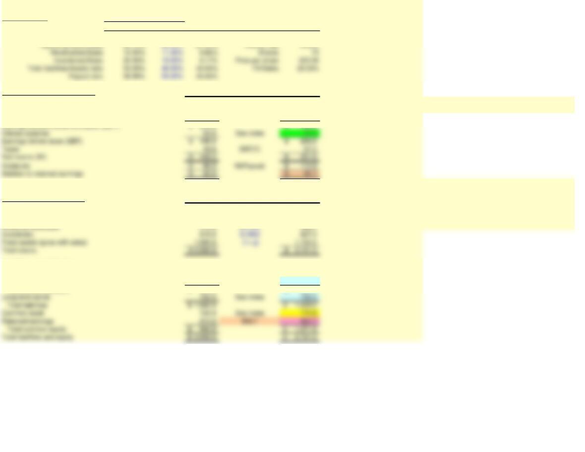
Table 16.2 Forecasted Financial Statements (Total dollars and shares in Millions) 12/12/2018
Part I. Inputs
2019 2020 Industry
Growth rate, g NA 10.00% NA Tax rate (T) 25.00%
Operating costs/Sales 90.73% 89.50% 87.00% Interest rate 9.60%
Part II. Income Statements 2019 Change 2020
Sales 3,000.0$ (1+ g) 3,300.0$
Operating costs (includes depreciation) 2,722.0 0.895 2,953.5
Earnings before interest and taxes (EBIT) 278.0$ 346.5$
Part III. Balance Sheets 2019 Change 2020
Assets
Cash (grow with sales) 10.0$ (1+ g) 11.0$
Accounts receivable 375.0 0.1100 363.0
Liabilities and Equity
Payables + accruals (both grow with sales) 200.0$ (1+ g) 220.0$
Short-term bank loans 110.0 See notes 103.5
Total current liabilities 310.0$ 323.5$
The primary “driver” for income statement changes is operating costs, which moves
toward the industry average: Op cost = New % × forecasted 2020 Sales.
Adjustable Inputs
Fixed Inputs
The “drivers” for the balance sheet changes are the changes in receivables and
inventories, which move toward the industry averages. The balancing items are bank
debt and common stock. The balancing procedure is explained in Part V, Notes on
Calculations.
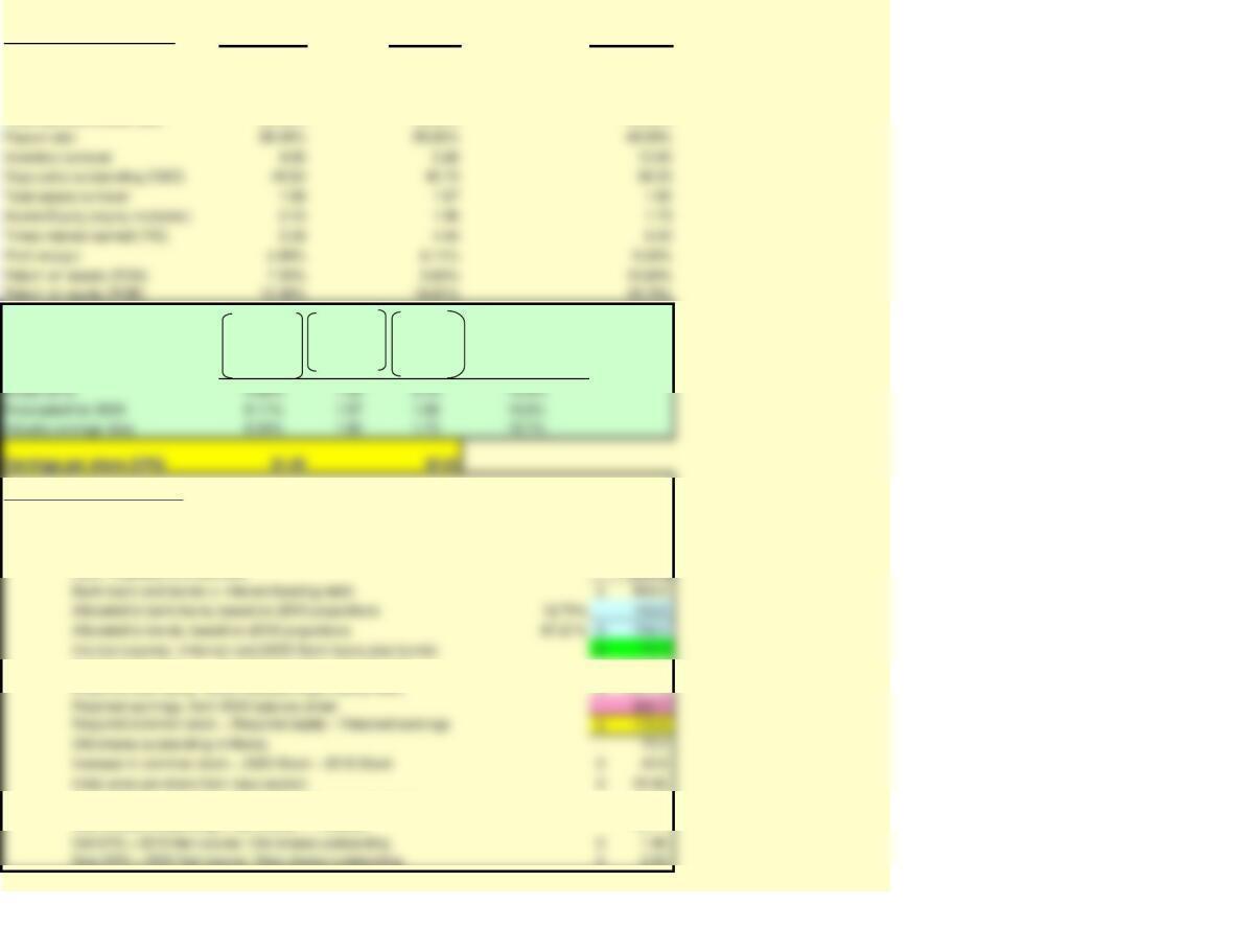
Part IV. Ratios and EPS 2019 2020E Industry
Operating costs/Sales 90.73% 89.50% 87.00%
Receivables/Sales 12.50% 11.00% 9.86%
Inventory/Sales 20.50% 19.00% 9.17%
Total liabilities/Assets ratio 53.00% 49.00% 40.00%
DuPont Calculations
Profit Margin
(NI/S)
Total Assets
Turnover
(S/A)
Equity
Multiplier
(A/ E)
= ROE
Part V. Notes on Calculations
Assets in 2020 will change to this amount, from the balance sheet 2,101.0$
Target total liabilities/assets ratio 49.00%
Resulting total liabilities: (Target total liabilities/assets ratio)( 2020 Assets) 1,029.5$
Less: Payables and accruals (220.0)
Target equity ratio = 1 – Target total liabilities/assets ratio 51.00%
Required total equity: (2020 Assets)(Target equity ratio) 1,071.5$
Change in shares = Change in stock/Initial price per share 1.77
New shares outstanding = Old shares + ∆ Shares 76.77
New EPS = 2020 Net income / New shares outstanding 2.63$
USING REGRESSION TO IMPROVE FORECASTS (Section 16-5) 12/12/2018
Year Sales Inventories Receivables
2015 $2,058 $387 $268
2016 2,534 398 297
2020 3,300 ? ?
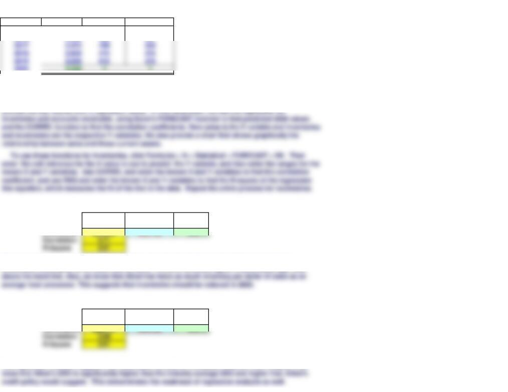
Forecasting Inventories
Regression Prior
Forecast Forecast Difference
Inventories $578.23 $627.00 -$48.77
R-Square 0.51
Forecasting Accounts Receivable
Regression Prior
Forecast Forecast Difference
Receivables $381.17 $363.00 $18.17
R-Square 0.81
Excel has a full-blown regression tool that can be accessed on the Data tab under Data Analysis. (If
you can’t see this on your screen, you will need to add Excel’s Analysis ToolPak add-in program.)
However, Excel has easier-to-use statistical functions (access through Formulas tab under fx) that
The regression forecast for inventories is lower than the original forecast, which assumed that
inventories would grow at the same rate as sales. The 2019 inventory figure is abnormally high, well
The regression forecast suggests that receivables should be increased; however, from Chapter 4 we
2017 2,472 409 304
2018 2,850 415 315
2019 3,000 615 375