243
CHAPTER 16
Externalities and Public Goods
A. Summary
Externalities were first introduced explicitly in Chapter 10. This chapter
provides a more detailed analysis of them. In defining externalities, actual
physical interactions are stressed. Following standard practice, external ef-
fects that operate through the market are not termed “externalities.” Principal
attention in the chapter is directed toward ways of coping with externalities.
The classical taxation and merger solutions are first presented. This is fol-
lowed by an extended discussion of the possibilities for bargaining, ending
with the Coase Theorem. When bargaining costs are high, externalities may
B. Lecture and Discussion Suggestions
Two lecture suggestions might be offered for this chapter. In discussing the
Coase Theorem, Meade’s bee-apple orchard example is very instructive.
Several articles have re-analyzed Meade’s fable and demonstrated that, in
fact, well developed markets in bee rental exist. Students seem to enjoy the
bucolic triviality of these bee examples. Alternatively, one might focus on a
Chapter 18: Externalities and Public Goods
244
wealth of material from the public choice literature. Tax limitation provisions
(Application 16.7) seem a particularly thought-provoking topic.
C. Glossary Entries in the Chapter
• Coase Theorem
• Common Property
• Externality
• Free Rider
• Lindahl Equilibrium
SOLUTIONS TO CHAPTER 16 PROBLEMS
16.1 a. MC = .4q. P = $20. Set P = MC.
20 = .4q, q = 50.
c. The graph shows the optimal tax in this widget market.
16.2 a. Fishers will arrange themselves so that the average catch on each lake is the
same. Since the average on lake Y is always 5, it must be 5 on lake X also. So
b. To maximize the catch, should set marginal productivities equal
Chapter 18: Externalities and Public Goods
245
c. The license fee should be set so that the average catch on lake X minus the fee
is equal to 5 (the catch on Y) when 5 fishers use the lake (the optimal number).
In this way, fishers themselves will opt for the correct allocation.
16.3 AC = MC = 10,000/well.
a. Produce where revenue/well = 10,000 = 100q = 50,000 – 100N. N = 400. There
is an externality here because drilling another well reduces output in all wells.
16.4 a. Suppose that equipment causes expected damage of d. With full information,
the equilibrium would be independent of legal rules. Suppose demanders in-
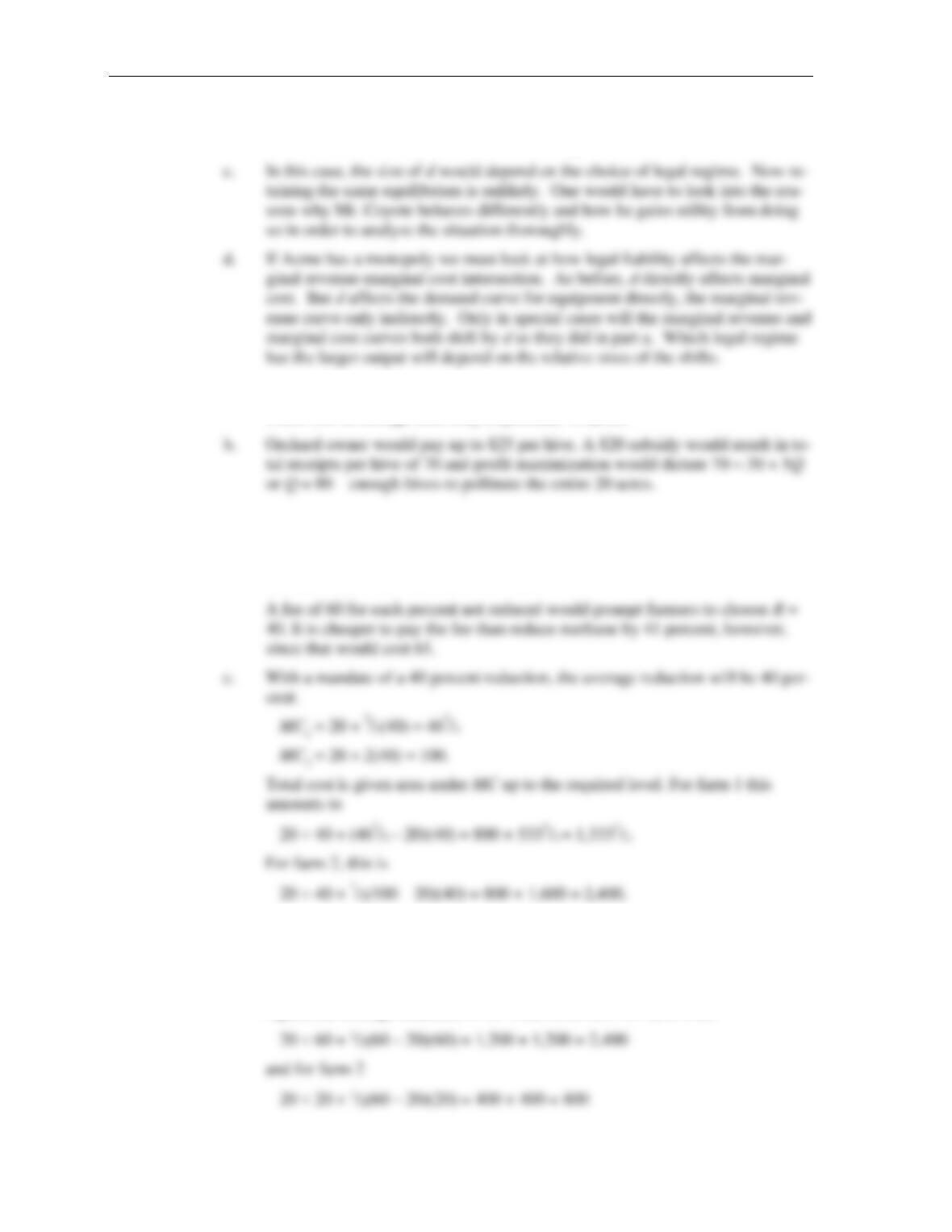
curred all costs – the equilibrium is shown by P*,Q* in the figure. Now if sup-
pliers are required to pay the damage costs, the supply curve would shift up by
d as would the demand curve (because buyers now have their costs reim-
bursed). Equilibrium would stay at Q*.
Chapter 18: Externalities and Public Goods
246
b. There would be no change because all parties fully expect Mr. Coyote to be
careless and use that information in assessing d.
16.5 a. For profit maximization, set P = MC, 50 = 30 + .5Q. Hence, Q = 40 hives.
There will be enough bees only to pollinate 10 acres.
16.6 a. Setting MB = MC yields 100 – R = 20 + R or R = 40.
b. The fee should be set so that farmers choose R = 40.
So, Fee = MC = 20 + R = 20 + 40 = 60.
So total costs of achieving the 40 percent reduction are 3,7331/3.
d. With a fee of 60, farm 1 sets 60 = 20 + 2/3R, and calculates R1 = 60.
Farm 2 calculates 60 = 20 + 2R2 or R2 = 20.
Again, the average reduction is 40. Total costs now for farm 1 are
Chapter 18: Externalities and Public Goods
247
16.7 a. Marginal valuation for person A = P = 100 – qA; for B, Marginal valuation = P
= 200 – qB. Because of the public good nature of mosquito control these should
be added “vertically.”
16.8 a. Total Net Benefits = $340 > $300. Under equal sharing A and B would vote for
the project, C against it. Net benefits for person A = 50, for person B = 40, and
for person C = –50.
16.9 a. The pool is nonrival (by assumption), but exclusion is possible.
b. Building the pool would generate $6,000 per day in economic value at a cost of
$5,000 per day. It would be efficient to build it.
c. A price of $3 would generate $3,000 in revenue, a price of $2 would generate
$4,000, and a price of $1 would generate $3,000. Obviously a price of $0
Chapter 18: Externalities and Public Goods
248
16.10 a. Since Q = 200 – 100P, profit maximizing price is .5(2 + .50) = 1.25. At this
price, Q = 75, p = (1.25 – .5)(75) = 56.25. Firm will be willing to pay up to this
amount per period as a bribe.