187
CHAPTER 15
TEACHING NOTES
When I wrote the first edition, I took the novel approach of introducing instrumental variables as
The omitted variable problem is conceptually much easier than simultaneity, and stating the
conditions needed for an IV to be valid in an omitted variable context is straightforward.
Besides, most modern applications of IV have more of an unobserved heterogeneity motivation.
The asymptotics underlying the simple IV estimator are no more difficult than for the OLS
estimator in the bivariate regression model. Certainly consistency can be derived in class. It is
also easy to demonstrate how, even just in terms of inconsistency, IV can be worse than OLS if
the IV is not completely exogenous.
Testing for endogeneity and testing any overidentification restrictions is something that should
be covered in second semester courses. The tests are fairly easy to motivate and are very easy to
implement.
188
SOLUTIONS TO PROBLEMS
15.1 (i) It has been fairly well established that socioeconomic status affects student performance.
The error term u contains, among other things, family income, which has a positive effect on
GPA and is also very likely to be correlated with PC ownership.
(ii) Families with higher incomes can afford to buy computers for their children. Therefore,
(iii) This is a natural experiment that affects whether or not some students own computers.
Some students who buy computers when given the grant would not have without the grant.
15.2 (i) It seems reasonable to assume that dist and u are uncorrelated because classrooms are not
usually assigned with convenience for particular students in mind.
(iii) We now need instrumental variables for atndrte and the interaction term,
priGPAatndrte. (Even though priGPA is exogenous, atndrte is not, and so priGPAatndrte is
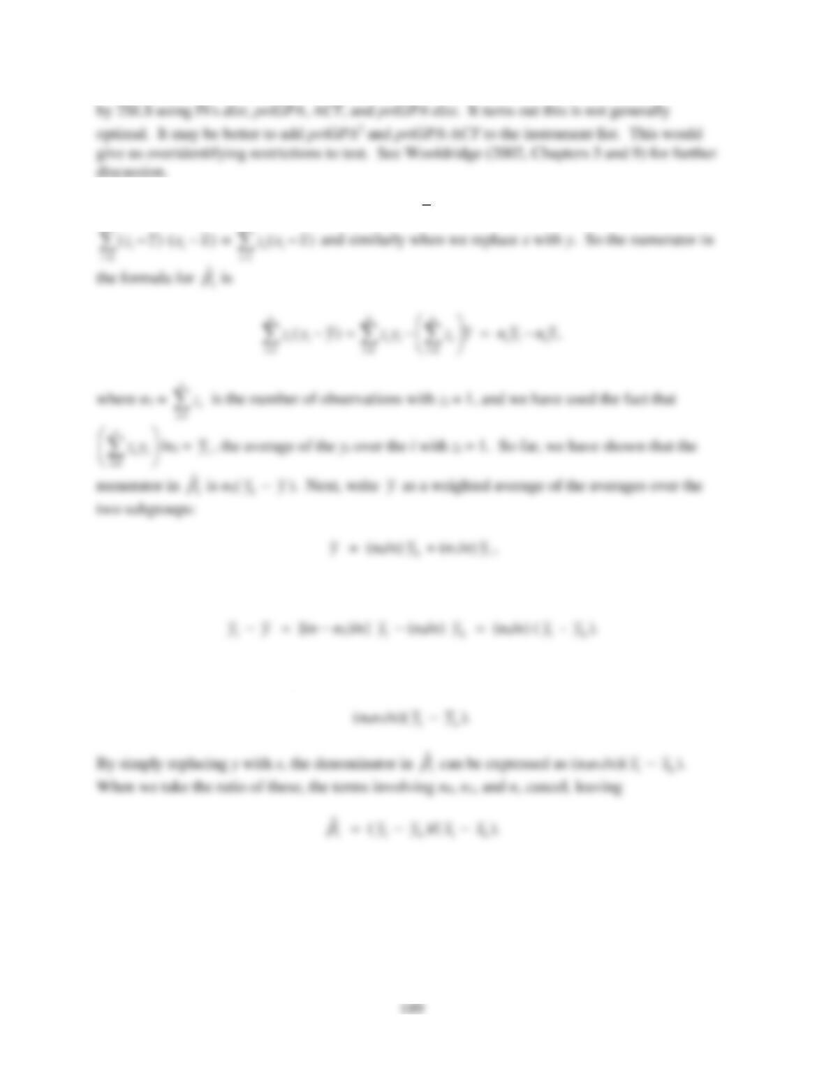
15.3 It is easiest to use (15.10) but where we drop
z
. Remember, this is allowed because
n
n
where n0 = n – n1. Therefore,
Therefore, the numerator of
1
ˆ
can be written as
15.4 (i) The state may set the level of its minimum wage at least partly based on past or expected
current economic activity, and this could certainly be part of ut. Then gMINt and ut are
correlated, which causes OLS to be biased and inconsistent.
190
15.5 (i) From equation (15.19) with
u =
x, plim
ˆ
=
1 + (.1/.2) =
1 + .5, where
ˆ
is the IV
15.6 (i) Plugging (15.26) into (15.22) and rearranging gives
(ii) From the equation in part (i), v1 = u1 +
1v2.
(iii) By assumption, u1 has zero mean and is uncorrelated with z1 and z2, and v2 has these
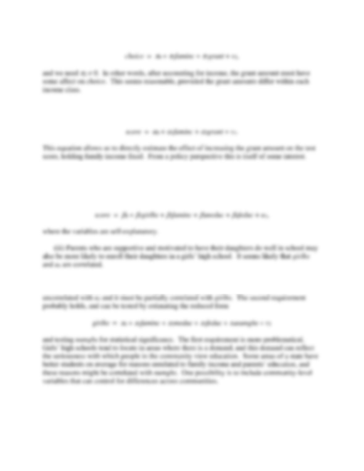
15.7 (i) Even at a given income level, some students are more motivated and more able than
others, and their families are more supportive (say, in terms of providing transportation) and
191
(iv) The reduced form for score is just a linear function of the exogenous variables (see
Problem 15.6):
score =
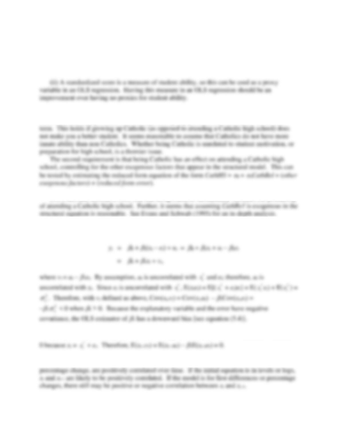
15.8 (i) A few examples include family income and background variables, such as parents’
education.
(ii) The population model is
score =
(iv) Let numghs be the number of girls’ high schools within a 20–mile radius of a girl’s
home. To be a valid IV for girlhs, numghs must satisfy two requirements: it must be
15.9 Just use OLS on an expanded equation, where SAT and cumGPA are added as proxy
variables for student ability and motivation; see Chapter 9.
192
15.10 (i) Better and more serious students tend to go to college, and these same kinds of students
may be attracted to private and, in particular, Catholic high schools. The resulting correlation
between u and CathHS is another example of a self-selection problem: students self select
toward Catholic high schools, rather than being randomly assigned to them.
(iii) The first requirement is that CathRe1 must be uncorrelated with unobserved student
motivation and ability (whatever is not captured by any proxies) and other factors in the error
(iv) Evans and Schwab (1995) find that being Catholic substantially increases the probability
15.11 (i) We plug
*
t
x
= xt – et into yt =
0 +
1
*
t
x
*
t
x
*
t
x
*
t
x
+ ut:
(ii) By assumption E(
*1t
x−
ut) = E(et-1ut) = E(
*1t
x−
et) = E(et-1et) = 0, and so E(xt-1ut) = E(xt-1et) =
(iii) Most economic time series, unless they represent the first difference of a series or the
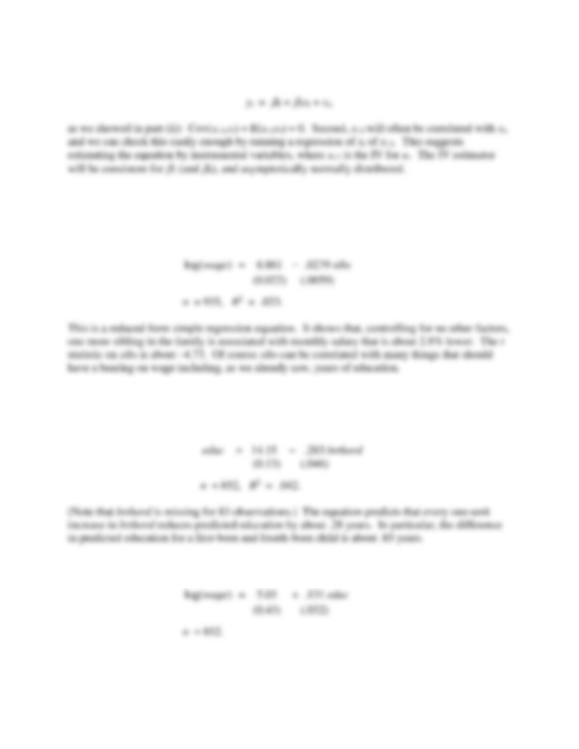
193
(iv) Under the assumptions made, xt-1 is exogenous in
SOLUTIONS TO COMPUTER EXERCISES
C15.1 (i) The regression of log(wage) on sibs gives
(ii) It could be that older children are given priority for higher education, and families may
hit budget constraints and may not be able to afford as much education for children born later.
The simple regression of educ on brthord gives
(iii) When brthord is used as an IV for educ in the simple wage equation we get
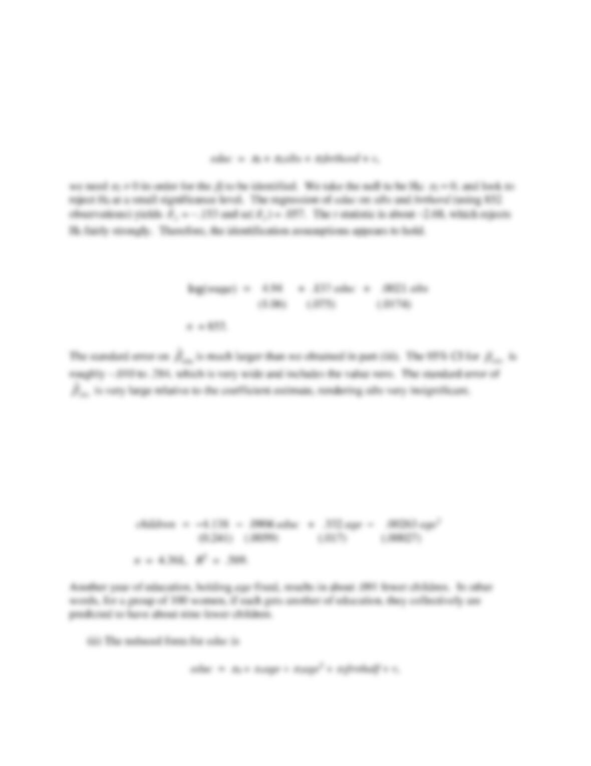
194
(The R-squared is negative.) This is much higher than the OLS estimate (.060) and even above
the estimate when sibs is used as an IV for educ (.122). Because of missing data on brthord, we
are using fewer observations than in the previous analyses.
(iv) In the reduced form equation
(v) The equation estimated by IV is
(vi) Letting
i
educ
be the first-stage fitted values, the correlation between
i
educ
and sibsi is
about −.930, which is a very strong negative correlation. This means that, for the purposes of
using IV, multicollinearity is a serious problem here, and is not allowing us to estimate educ with
much precision.
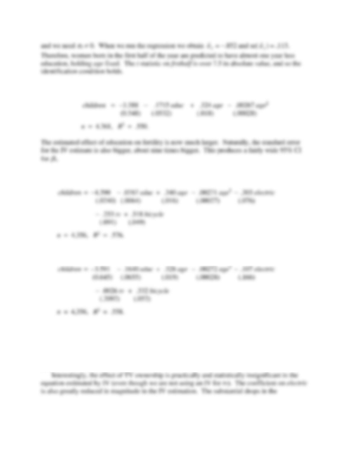
C15.2 (i) The equation estimated by OLS is
195
(iii) The structural equation estimated by IV is
(iv) When we add electric, tv, and bicycle to the equation and estimate it by OLS we obtain
The 2SLS (or IV) estimates are
Adding electric, tv, and bicycle to the model reduces the estimated effect of educ in both cases,
but not by too much. In the equation estimated by OLS, the coefficient on tv implies that, other
factors fixed, four families that own a television will have about one fewer child than four
families without a TV. Television ownership can be a proxy for different things, including
income and perhaps geographic location. A causal interpretation is that TV provides an
alternative form of recreation.
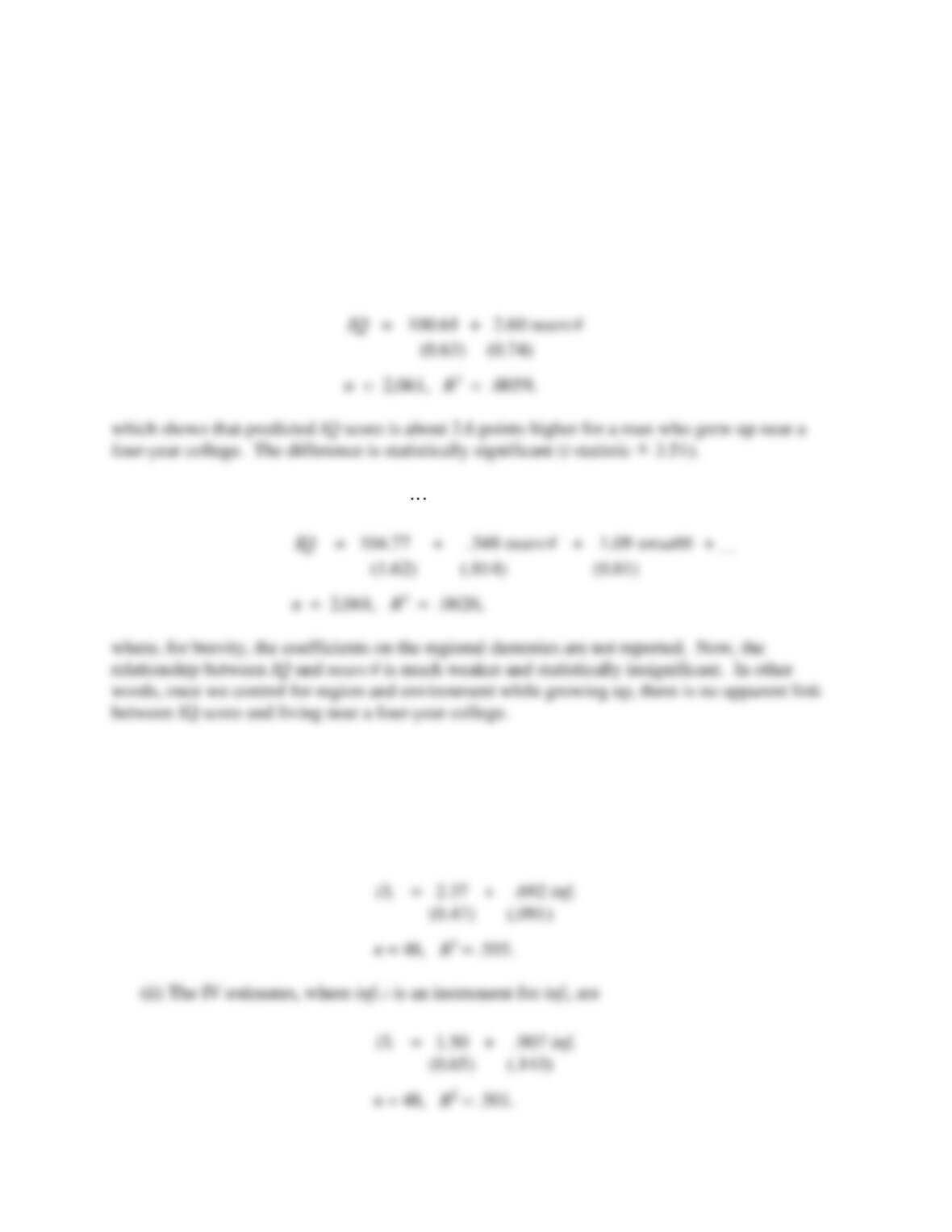
196
magnitudes of these coefficients suggest that a linear model might not be the best functional
form, which would not be surprising since children is a count variable. (See Section 17.4.)
C15.3 (i) IQ scores are known to vary by geographic region, and so does the availability of four
year colleges. It could be that, for a variety of reasons, people with higher abilities grow up in
areas with four year colleges nearby.
(ii) The simple regression of IQ on nearc4 gives
(iii) When we add smsa66, reg662, , reg669 to the regression in part (ii), we obtain
(iv) The findings from parts (ii) and (iii) show that it is important to include smsa66, reg662,
…, reg669 in the wage equation to control for differences in access to colleges that might also be
correlated with ability.
C15.4 (i) The equation estimated by OLS, omitting the first observation, is
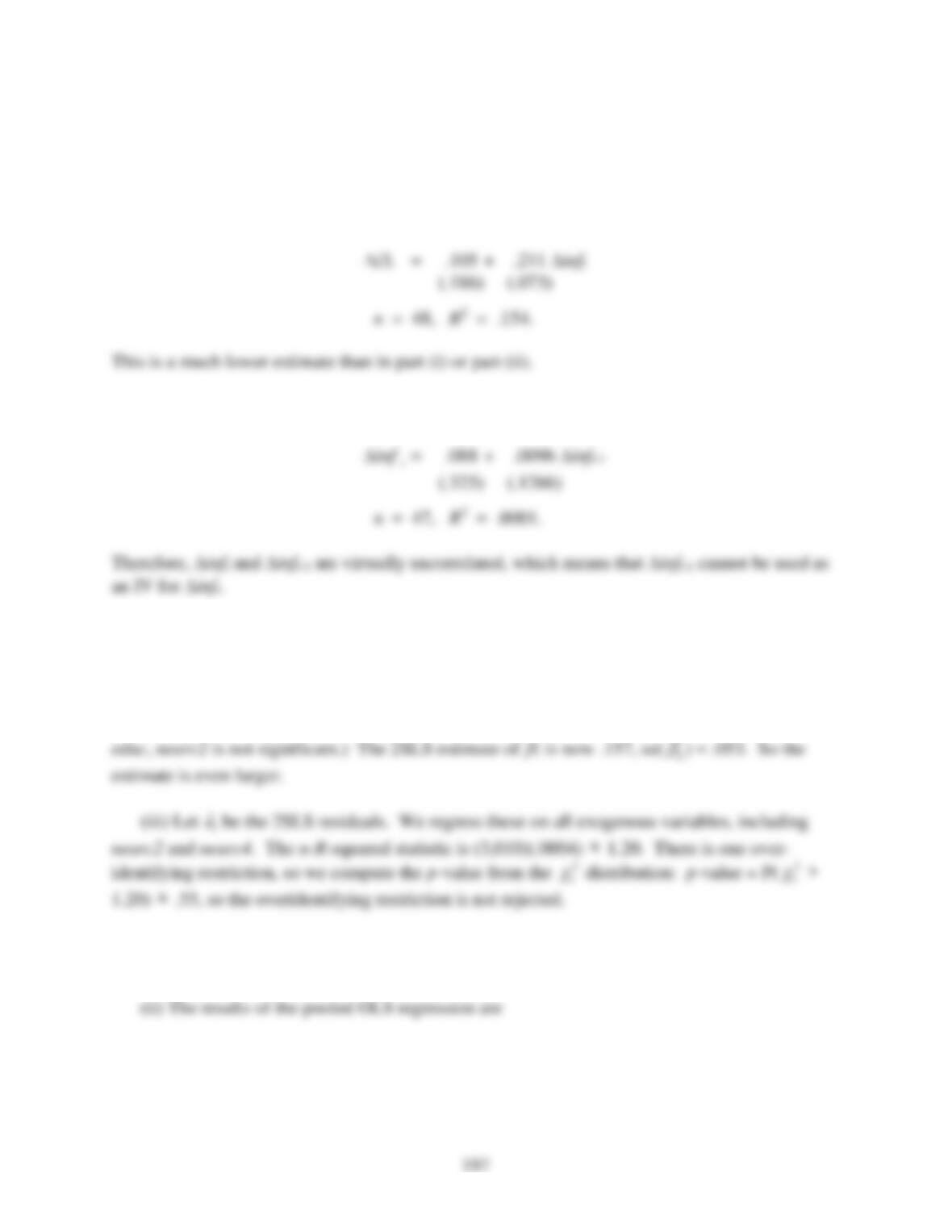
The estimate on inft is no longer statistically different from one. (If
1 = 1, then one percentage
point increase in inflation leads to a one percentage point increase in the three-month T-bill rate.)
(iii) In first differences, the equation estimated by OLS is
(iv) If we regress inft on inft-1 we obtain
C15.5 (i) When we add
2
ˆ
v
to the original equation and estimate it by OLS, the coefficient on
2
ˆ
v
is about –.057 with a t statistic of about –1.08. Therefore, while the difference in the estimates of
the return to education is practically large, it is not statistically significant.
(ii) We now add nearc2 as an IV along with nearc4. (Although, in the reduced form for
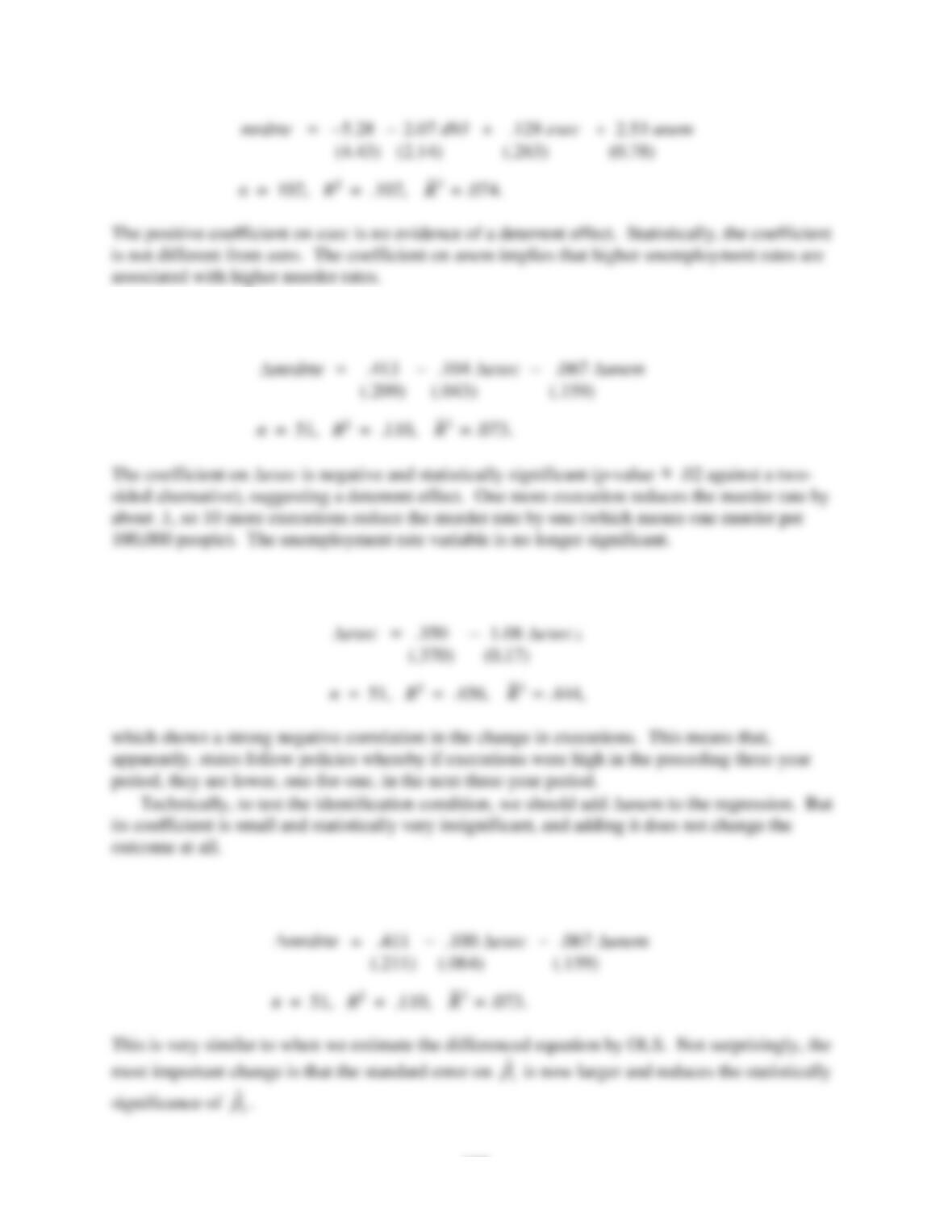
C15.6 (i) Sixteen states executed at least one prisoner in 1991, 1992, or 1993. (That is, for 1993,
exec is greater than zero for 16 observations.) Texas had by far the most executions with 34.
198
(iii) When we difference (and use only the changes from 1990 to 1993), we obtain
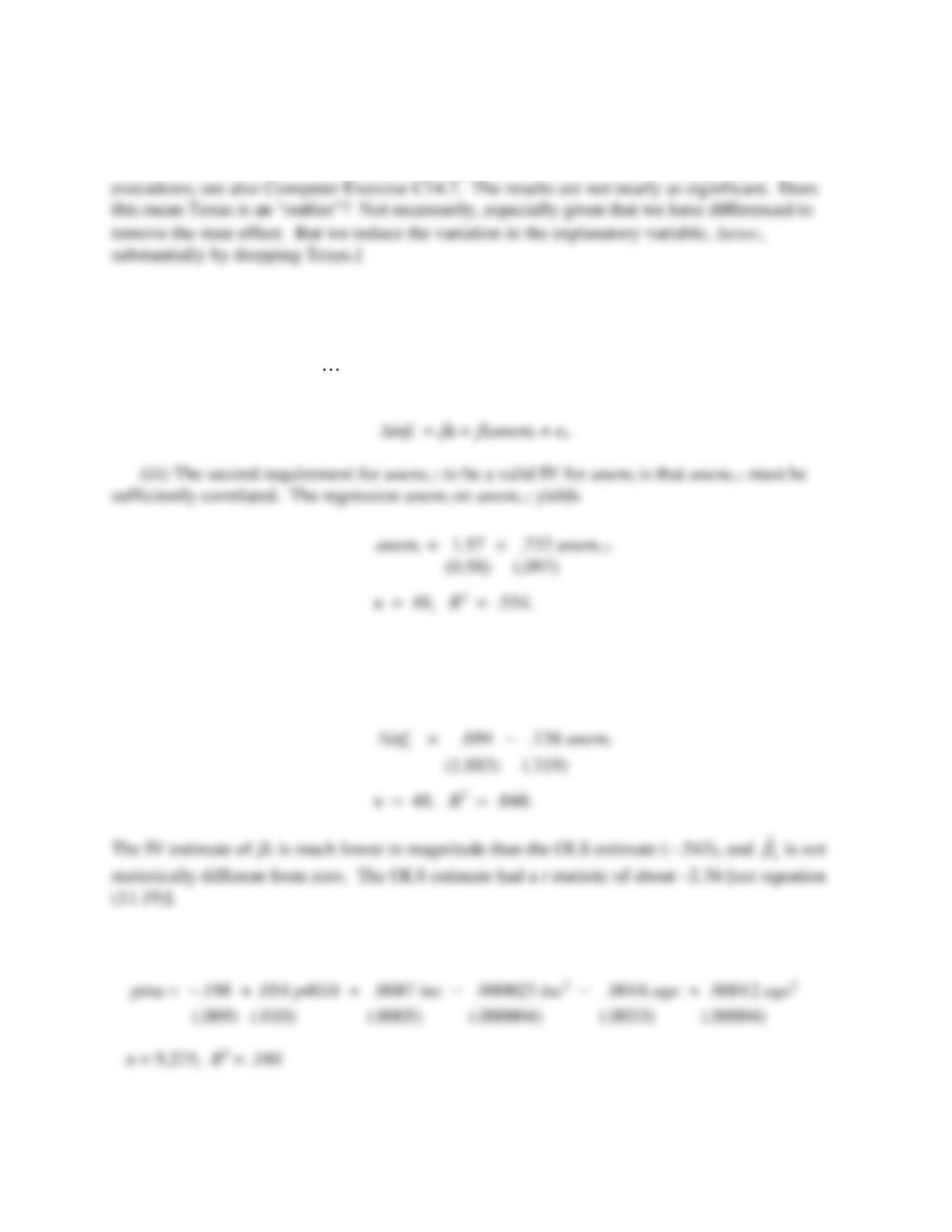
(iv) The regression exec on exec-1 yields
(v) When the differenced equation is estimated using exec-1 as an IV for exec, we obtain
199
[Instructor’s Note: As an illustration of how important a single observation can be, you might
want the students to redo this exercise dropping Texas, which accounts for a large fraction of
C15.7 (i) As usual, if unemt is correlated with et, OLS will be biased and inconsistent for
estimating
1.
(ii) If E(et|inft-1,unemt-1, ) = 0 then unemt-1 is uncorrelated with et, which means unemt-1
satisfies the first requirement for an IV in
Therefore, there is a strong, positive correlation between unemt and unemt-1.
(iv) The expectations-augmented Phillips curve estimated by IV is
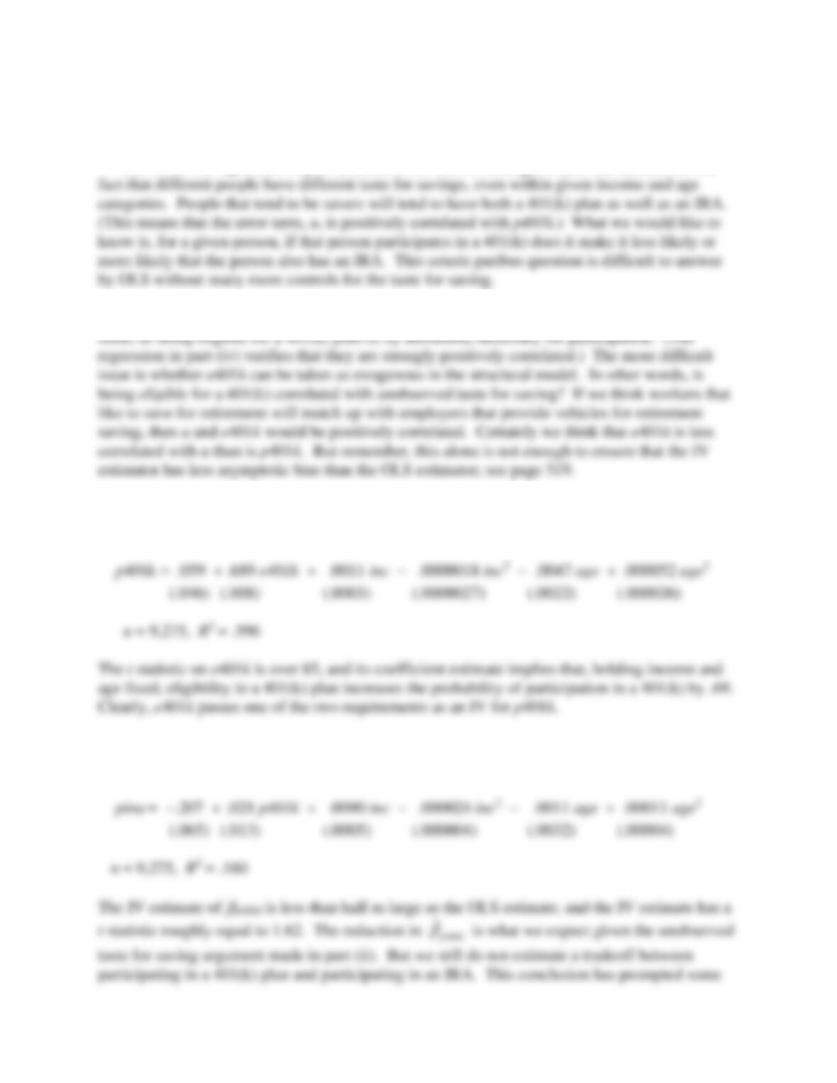
C15.8 (i) The OLS results are
200
The coefficient on p401k implies that participation in a 401(k) plan is associate with a .054
higher probability of having an individual retirement account, holding income and age fixed.
(ii) While the regression in part (i) controls for income and age, it does not account for the
(iii) First, we need e401k to be partially correlated with p401k; not surprisingly, this is not an
(iv) The reduced form equation, estimated by OLS but with heteroskedasticity-robust
standard errors, is
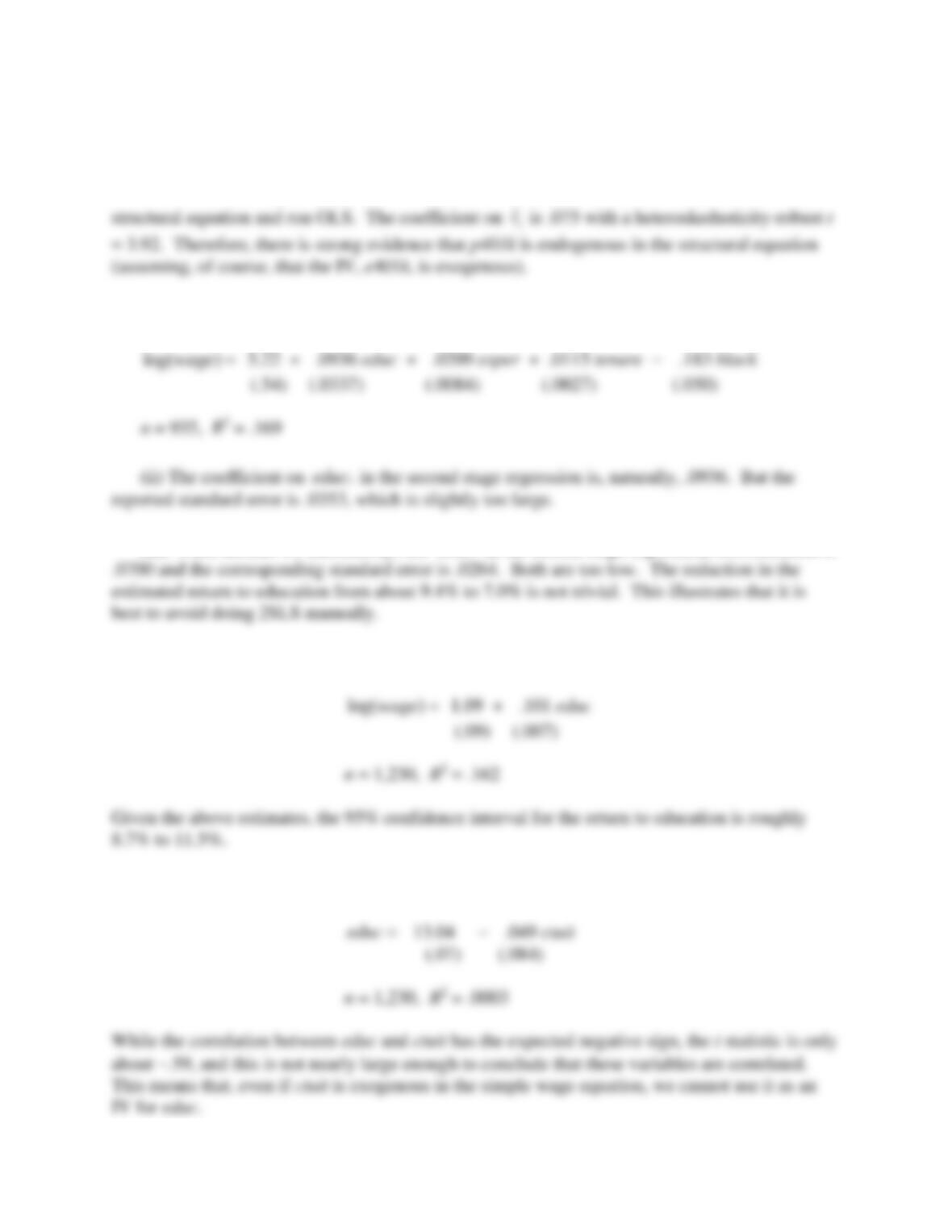
(v) When e401k is used as an IV for p401k we get the following, with heteroskedasticity-
robust standard errors:
201
in the literature to claim that 401(k) saving is additional saving; it does not simply crowd out
saving in other plans.
(vi) After obtaining the reduced form residuals from part (iv), say
ˆi
v
, we add these to the
C15.9 (i) The IV (2SLS) estimates are
(iii) When instead we (incorrectly) use
i
educ
in the second stage regression, its coefficient is
C15.10 (i) The simple regression gives
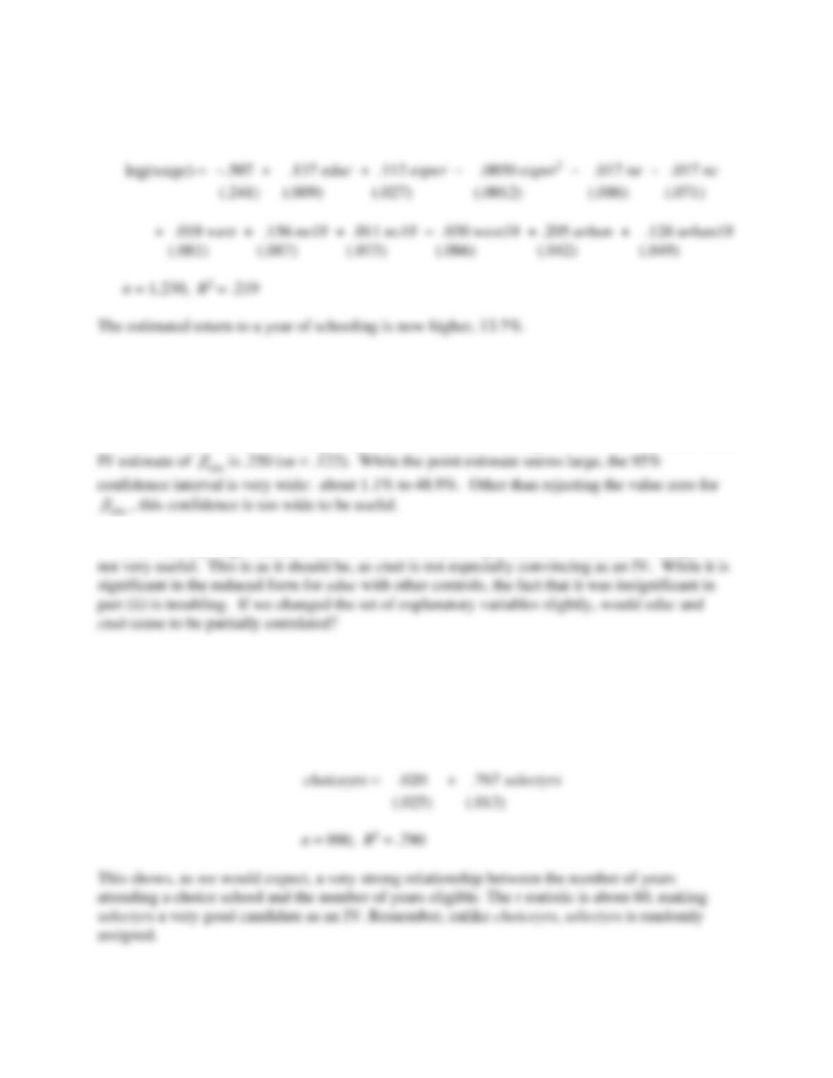
(ii) The simple regression of educ on ctuit gives
202
(iii) The multiple regression equation, estimated by OLS, is
(iv) In the multiple regression of educ on ctuit and the other explanatory variables in part
(iii), the coefficient on ctuit is −.165, t statistic = −2.77. So an increase of $1,000 in tuition
reduces years of education by about .165 (since the tuition variables are measured in thousands).
(v) Now we estimate the multiple regression model by IV, using ctuit as an IV for educ. The
(vi) The very large standard error of the IV estimate in part (v) shows that the IV analysis is
C15.11 (i) We look at the variables selectyrs and choiceyrs. From selectyrs, out of 990 students,
468 were never awarded a voucher and 108 were selected in the voucher system for all four
years. From choiceyrs, only 56 actually attended a choice school for four years.
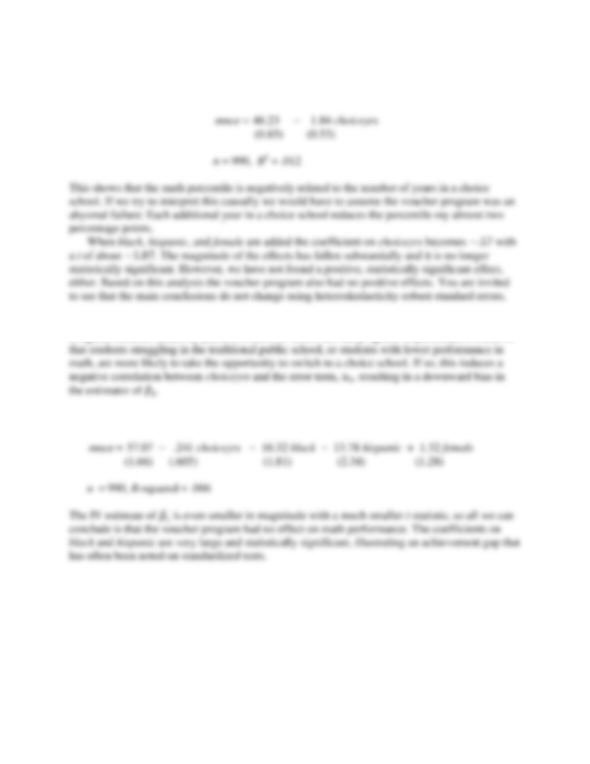
(ii) The estimated equation, with usual OLS standard errors in parentheses, is
203
(iii) Regressing mnce on choiceyrs gives the following (usual OLS standard errors in
parentheses):
(iv) Even controlling for race, ethnicity, and gender, and even with the vouchers randomly
assigned, students (aided by parents) could self-select into the program. In particular, it could be
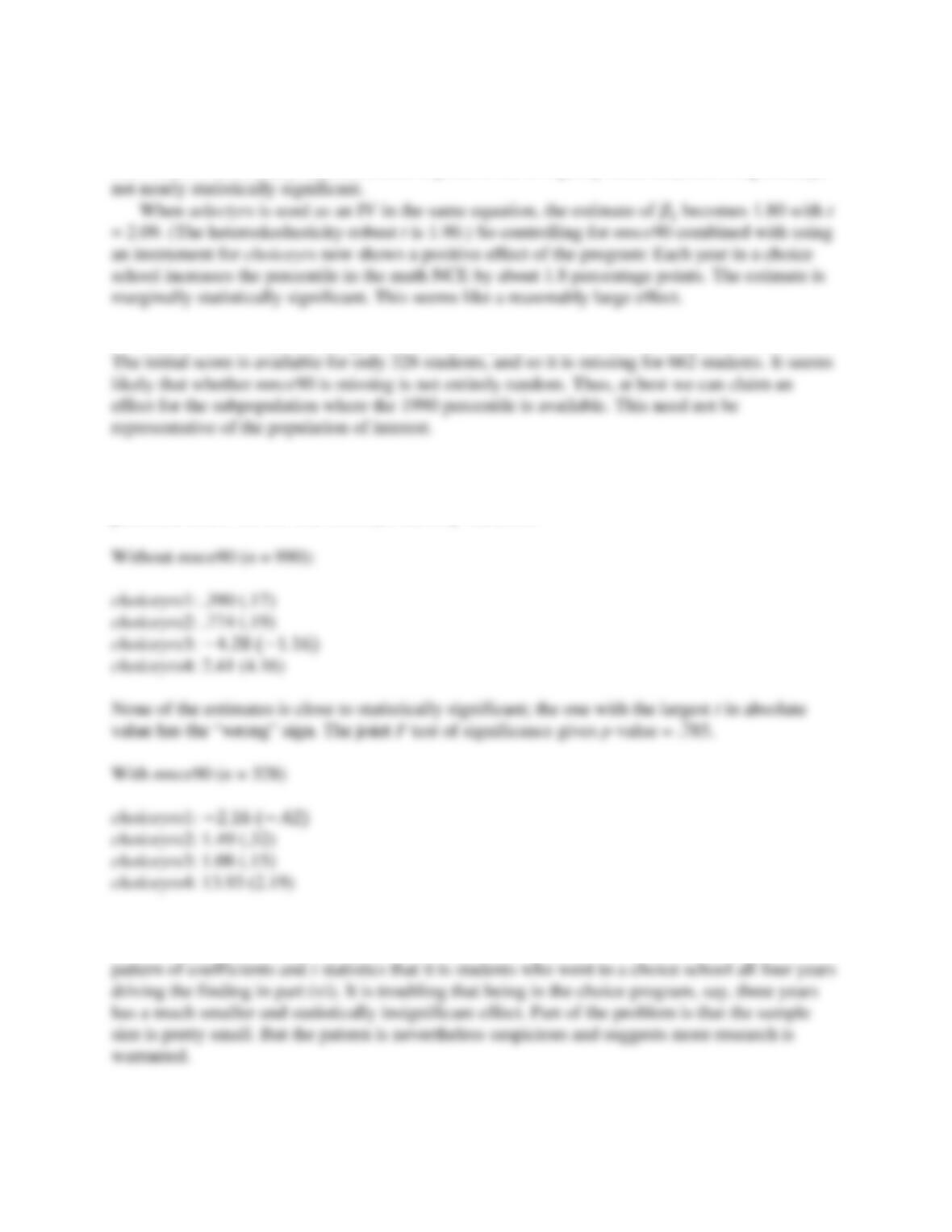
(v) The IV estimates are given by
204
(vi) When mnce90 is added to the equation, and OLS is used, the estimate of 𝛽1 becomes
.411 with t = .56. So now the coefficient is positive but it is pretty small and, more importantly,
(vii) Unfortunately, including mnce90 in the equation results in a severe loss of observations:
(viii) There is a typo in the first printing of the text. The equation should include mnce90,
although it is useful to see what happens without it, too. The IV estimates and t statistics are
presented below for the four choiceyrs dummy variables.
The coefficient on choiceyrs4 is huge – a 14 percentage point move up in the math score
distribution – but it is imprecisely estimated (with a marginal t statistic). It is clear from the