359
LECTURE SUPPLEMENT
15–1 How a Real Business Cycle Model Is Constructed
The dynamic AD–AS model developed in this chapter can be used to analyze economic growth by
considering how an increase in the natural level of output affects the economy. While this feature can be
interpreted as incorporating a long–run growth path for the economy into a model of short–run fluctuations,
it can also be interpreted as allowing for elements of the real business cycle approach (discussed in the
appendix to Chapter 9) to play a role in short–run business cycle analysis. In this sense, the model of
Chapter 15 can be viewed as a hybrid model that includes both Keynesian features that allow money to
have short–run real effects and real business cycle elements that influence short–run fluctuations. The more
advanced dynamic, stochastic, general equilibrium (DSGE) models mentioned in the text also exhibit
these hybrid characteristics. This supplement and the several to follow discuss how real business cycle
models are constructed and tested.
Real business cycle models emphasize the role of technology shocks in driving short–run economic
fluctuations. These models generally differ from other macroeconomic models, not only in their
theoretical explanation of economic fluctuations, but also in the way they are tested with economic data.
Typically, economists test a theory by ascertaining an implication of that theory for economic data and
1 C. Plosser, “Understanding Real Business Cycles,” Journal of Economic Perspectives 3, no. 3 (Summer 1989): 51–77.
2 If the economy is competitive (as Plosser assumes), then markets will allocate resources efficiently and we will not be badly misled by simply
360
361
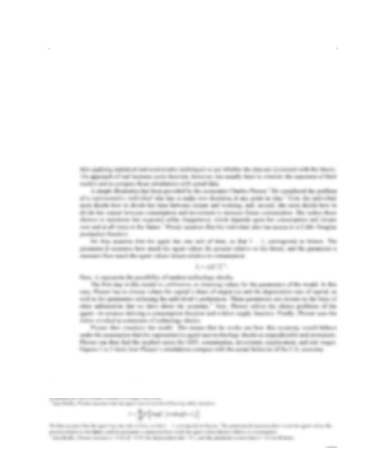
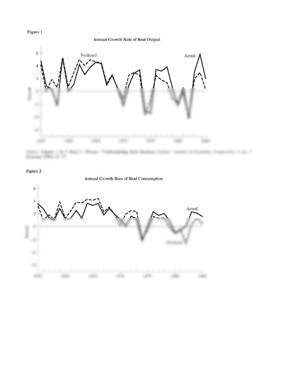
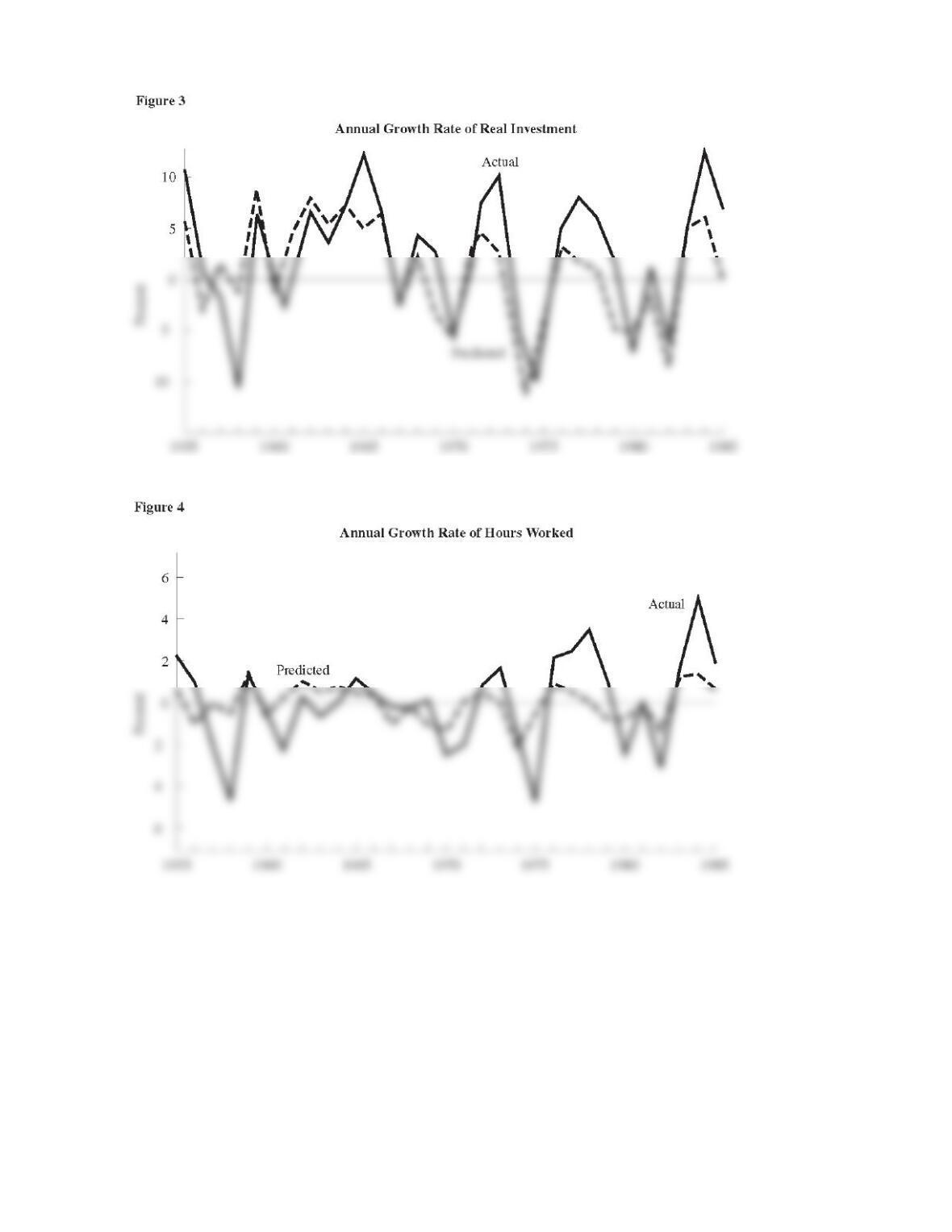
Interpreting these figures is not easy, but they are quite striking. In particular, Plosser’s simulations
for output and consumption seem to match up very well with the actual data, although the fit is worse for
investment and labor market variables. These pictures indicate that a competitive economy hit by
technology shocks can exhibit fluctuations that broadly resemble those experienced by the U.S. economy.
A problem with this line of research is that there has been insufficient formal statistical analysis of
what constitutes a good match between simulated results and actual data. Plosser’s simulations look as if
they correspond to the U.S. data, but we cannot tell from inspection whether there is a good fit in a more
formal statistical sense. Also, as discussed in Chapter 9 of the textbook, the Solow residual may not be a
5 See also Supplement 8–3, “Does the Solow Model Really Explain Japanese Growth?” for another use of a real business cycle model. That
LECTURE SUPPLEMENT
15–2 The Microeconomics of Labor Supply
Many economists are unconvinced that real business cycle theory can adequately explain fluctuations in
employment. To pursue this further, we start from two features of this theory: first, prices are assumed to
be flexible; and, second, shocks to technology are the driving force behind economic fluctuations.
Since prices are flexible, it follows that the labor market is always in equilibrium, so labor demand
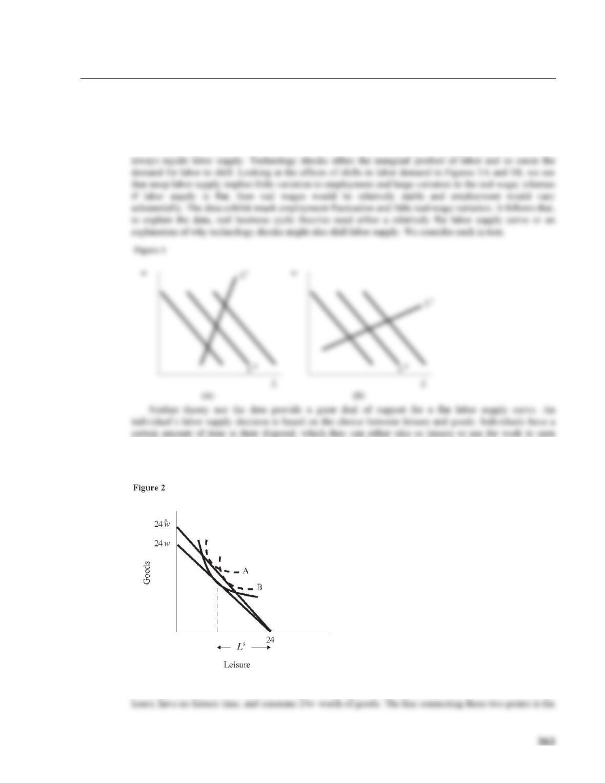
income with which to buy goods. The real wage, w, is the relative price of leisure in terms of goods. The
higher the real wage, the more goods must be forgone for an extra hour of leisure. We illustrate this in the
standard microeconomic manner in Figure 2.
We suppose that the individual has 24 hours to allocate between working and leisure. At one extreme,
she could not work at all and take all her time as leisure. At the other extreme, she could work all 24
theoretically ambiguous. It is perhaps not surprising that the data show that changes in the real wage do
not have strong effects on labor supply. In terms of our original diagrams, therefore, the labor supply curve
is steep. Contrary to the data, we would expect to see large changes in the real wage and small changes in
employment if the economy is competitive and characterized by changes in labor demand.
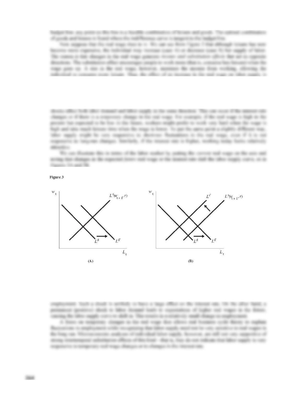
We observe a larger change in employment and a smaller change in the real wage if technology
An increase in the future real wage (wt + 1) makes the current supply of labor less attractive and so
causes the labor supply curve to shift inward. An increase in the interest rate is like a decrease in the future
real wage and so shifts the labor supply curve outward.
Now, consider a temporary shock to labor demand (caused perhaps by a temporary shock to the
technology). This shock does not affect the future real wage and so leads to a relatively large change in
365
LECTURE SUPPLEMENT
15–3 Quits and Layoffs
Job separations can occur either because workers voluntarily quit their jobs or because they are laid off (or
fired with cause). We can thus write
s = q + l,
where s is the separation rate (see Chapter 7), q is the quit rate, and l is the layoff rate. Theories of
intertemporal substitution argue that employment is lower in recessions because the real wage (or the
interest rate) falls and workers are unwilling to work at this lower wage. Such an explanation suggests that
quits should be an important component of flows from employment to unemployment, and also that quits
should be higher in recessions.
1 U.S. Department of Labor, Bureau of Labor Statistics.
LECTURE SUPPLEMENT
15–4 Involuntary Unemployment and Overqualification
Some economists distinguish between two types of unemployment: voluntary and involuntary. According
to the usual definition, someone is voluntarily unemployed if, at the existing wage, she does not think it
worthwhile to work. A person who is involuntarily unemployed would like to work at existing wages but
cannot obtain a job.
Other economists argue that the idea of involuntary unemployment makes no sense. After all, they
suggest, an unemployed investment banker or neurosurgeon could always get a job flipping hamburgers or
waiting tables. So how can we distinguish between involuntary and voluntary unemployment? Robert
Lucas expands on this argument as follows:1
Nor is there any evident reason why one would want to draw this distinction. Certainly the
more one thinks about the decision problem facing individual workers and firms the less sense
this distinction makes. The worker who loses a good job in prosperous times does not
volunteer to be in this situation; he has suffered a capital loss…. Nevertheless the unemployed
worker at any time can always find some job at once…. Thus there is an involuntary element in
all unemployment, in the sense that no one chooses bad luck over good; there is also a
voluntary element in all unemployment, in the sense that however miserable one’s current
work options, one can always choose to accept them.
Truman Bewley, an economist at Yale University, interviewed a large number of businesspeople to
learn more about their decisions about hiring workers. His findings suggest that it may not be quite so easy
for unemployed workers to find jobs, even at lower wages2:
ADVANCED TOPIC
15–5 Why Technology Shocks Are So Important in Real Business Cycle
Models
In any competitive flexible–price model, such as those espoused by real business cycle theorists, labor
market clearing implies that the real wage must equal the marginal product of labor. As explained in
Chapter 3, the marginal product of labor gives the firm’s demand for labor and depends upon the amount
of capital and labor that firms possess. In particular, we expect to see diminishing marginal product: the
marginal product of labor will be lower when employment is higher, absent other complications. We write
MPL(K, L) = W/P.
We know that employment is procyclical—not surprisingly, employment is higher in booms and
lower in recessions. Other things being equal, we would expect to see the marginal product of labor falling
in booms, and hence, if the economy is competitive, we would expect to see the real wage also being
lower in booms. But we also know from Case Studies 14-1 and 14-2 that the real wage is actually mildly
procyclical—real wages are higher in booms and lower in recessions.1
This says that, in a competitive economy, the price of output equals the marginal cost of production (since
the wage is the cost of a unit of labor and the marginal product of labor gives the amount of output
contributed by the last unit of labor). Under imperfect competition, however, firms set prices as a markup
(m) over marginal cost:
P = m × (W/MPL)
⇒ MPL/m = (W/P).
1 Procyclical real wages are also a necessary ingredient of real business cycle theory. If high employment in booms and low employment in
recessions arise from voluntary shifting of labor, it follows that workers are choosing to consume less leisure in booms and more leisure in
recessions. But why would they choose to consume less leisure and more consumption goods at the same time? The answer has to be that leisure is
ADVANCED TOPIC
15–6 Real Business Cycles and Random Walks
Real business cycle theory provides a challenge to the traditional explanation of macroeconomic
fluctuations. One reason why this theory has been so influential is the work of two economists, Charles
Nelson and Charles Plosser.
In an important article published in 1982, Nelson and Plosser argued that there is evidence to suggest
that U.S. GDP may follow a random walk.1 That is, they suggested that the behavior of real GDP over
time could be described by the equation
The conventional view of macroeconomic fluctuations is that the behavior of GDP over time can be
decomposed into a long–run natural–rate or trend component and a short–run cyclical component. This
approach underlies the models used in the textbook: The Solow growth model explains the long–run
behavior of the economy and the aggregate demand–aggregate supply model explains short–run
fluctuations. In this view, shocks to the economy will push it away from the natural rate only temporarily;
the economy always has a tendency to revert to the natural rate. But the Nelson–Plosser finding challenges
this characterization. If GDP does follow a random walk, then shocks to output have permanent effects.
To see this, suppose that at some time (t = 0), GDP is at the value Y0, and that at t = 1 there is a one–
unit shock to GDP (u1 = 1). Suppose also that there are no further shocks (u2 = u3 = . . . = 0). Then
Y1 = Y0 + 1.
Now
that technological progress is irregular and a source of fluctuations. Indeed, if this real business cycle
characterization of the data is accurate, then the traditional decomposition of output into cycle and trend
does not really make sense.
If GDP does not follow a random walk, then the conclusion is very different. Suppose, for example,
that the behavior of GDP can be described by the equation
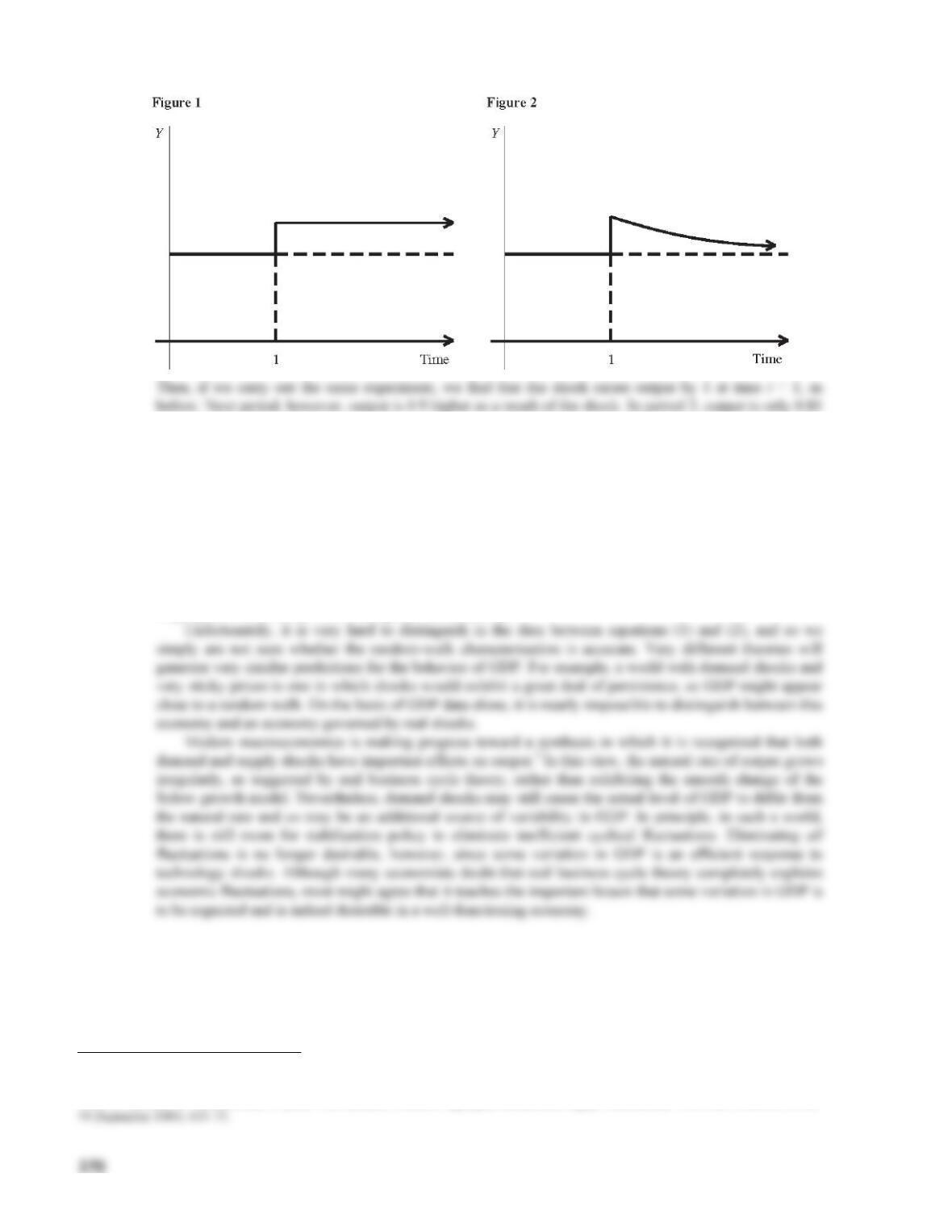
(= 0.92) units higher, and so on. In other words, the impact of the shock on GDP gradually dies out. In this
representation, shocks to the economy are temporary, not permanent, and output does tend to return to the
natural rate following a shock (Figure 2).
So, if the Nelson–Plosser result is right, and GDP can be well described by a random walk, we need to
think in terms of models where shocks have permanent effects. In terms of standard aggregate demand–
aggregate supply models, this suggests that real or supply shocks, such as to technology, govern the
behavior of GDP; aggregate demand shocks do not have permanent effects on output in such models.
Demand shocks may, however, have permanent effects on GDP in other models such as the hysteresis
models discussed in Chapter 14. Steve Durlauf, however, points out that if GDP follows a random walk, it
is also consistent with a world in which coordination failures are important. In this case, demand shocks
might push the economy from one equilibrium to another.2
2 S. Durlauf, “Output Persistence, Economic Structure and the Choice of Stabilization Policy,” Brookings Papers on Economic Activity 2 (1989): 69–
136.
3 See, for example, O. Blanchard and D. Quah, “The Dynamic Effects of Aggregate Demand and Supply Disturbances,” American Economic Review
LECTURE SUPPLEMENT
15–7 Inflation Inertia
The Phillips curve used in the dynamic AD–AS model of Chapter 15 can be derived under the assumption
that all firms have the ability to set prices and some of those firms set their prices one period in advance.
As shown in Chapter 14, this assumption implies a Phillips curve that relates period t inflation to the
period t – 1 expectation of period t inflation and the gap between actual and the natural level of output.
Introducing adaptive expectations then allows derivation of the DAS curve, which relates period t inflation
to period t – 1 inflation and the deviation in output from its natural level. The effect of lagged inflation in
the DAS curve is responsible in the model for the gradual adjustment of inflation in response to shocks.
The reason for this result is that when price–setters fix a price for the current and future periods, they
consider not only today’s overall price level but also the price level expected to prevail in the future. The
resulting Phillips curve expresses inflation as a function of next period’s inflation and the current output
gap. Accordingly, a declining path for inflation is associated with output above its natural rate.
Evidence for the United States and many other countries contradicts this implication and supports the
view that inflation is highly persistent. Periods of disinflation across countries are overwhelmingly periods
when output is below normal.2 And estimates of the inflation process for the United States find that lagged
inflation helps explain current inflation.3
Various ways of reconciling new Keynesian models of price dynamics with evidence of inflation
inertia have been proposed. These include adding delays in price adjustment, incorporating some
backward–looking price–setters, indexing fixed prices to overall inflation between adjustments, and
introducing more complex dynamics in costs or markups.
1994): 155–83.
3 See Jeffrey Fuhrer, “The (Un)Importance of Forward–Looking Behavior in Price Specifications,” Journal of Money, Credit, and Banking, 29
ADDITIONAL CASE STUDY
15–8 Volatility and Growth
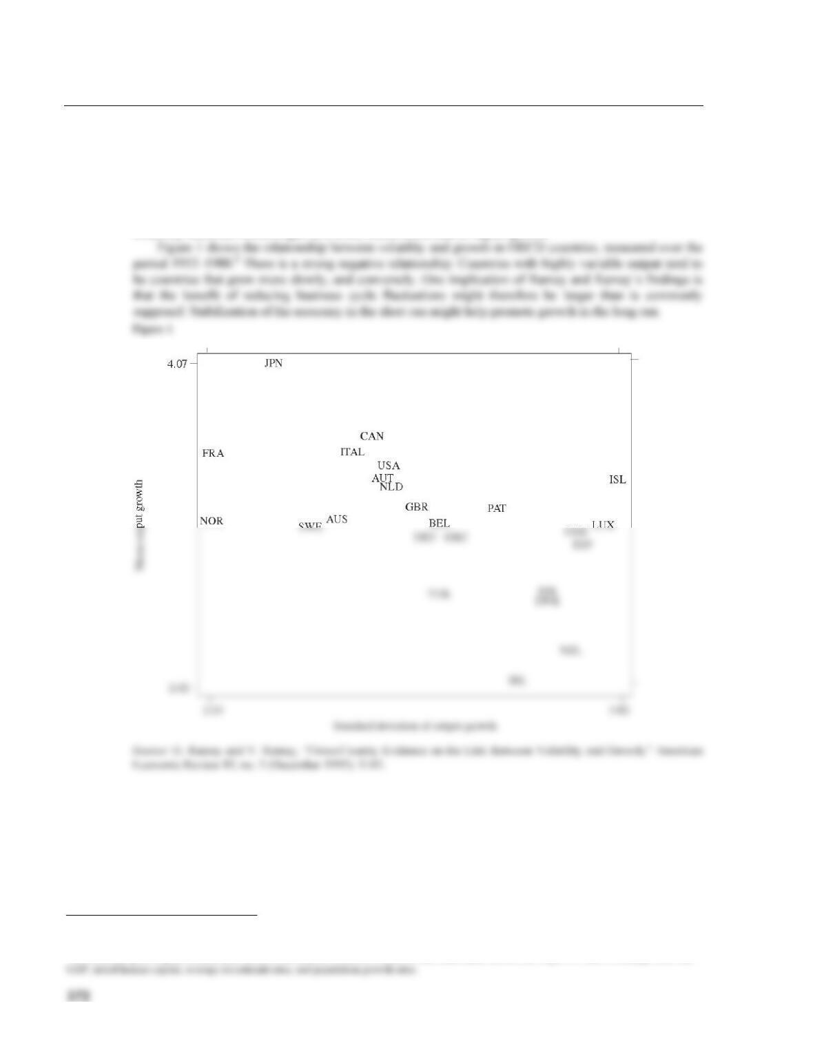
Garey Ramey and Valerie Ramey investigated the connection between the growth and the volatility of
GDP in a number of different countries.1 They wished to find out if long-run growth and short–run
volatility were related. As a matter of theory, growth and volatility could be directly or inversely related.
For example, large fluctuations in output might make firms reluctant to commit to irreversible investment,
implying that growth would be lower in countries with highly variable output. Conversely, consumers in a
relatively uncertain world might save a lot, which could lead to higher growth.
1 G. Ramey and V. Ramey, “Cross–Country Evidence on the Link Between Volatility and Growth,” American Economic Review 85, no. 5 (December
1995): 1138–51.
2 In constructing this figure, Ramey and Ramey controlled for a number of factors that could cause differences in growth rates, including initial real
373
LECTURE SUPPLEMENT
15–9 How Long Is the Long Run? Part Four
Macroeconomists traditionally decompose the overall behavior of GDP through time into its long–run
growth (or trend) and its short–run fluctuations (or cycle). That is the approach followed in the textbook.
Chapters 3, 6, 8, and 9 explain the determination of the natural level of output at a point in time and show
how the natural level of output grows through time as the economy’s resources and technology change.
Chapters 10 to 14 explain how actual GDP may differ from the natural level in the short run because of
shocks to aggregate demand combined with an upward–sloping aggregate supply curve (as a result of price
stickiness or information imperfections). Thus, Chapters 3, 6, 8, and 9 explain the trend growth of GDP,

374
LECTURE SUPPLEMENT
15–10 Additional Readings
The Summer 1989 issue of the Journal of Economic Perspectives 3, no. 3, contains two articles on real
business cycle theory: one by Charles Plosser, a proponent of the theory, “Understanding Real Business
Cycles,” pages 51–77; and one by Greg Mankiw, who is more skeptical, “Real Business Cycles: A
Keynesian Perspective,” pages 79–90. A useful, but more technical, survey is B. McCallum, “Real
Business Cycle Models,” in R. Barro (ed.), Modern Business Cycle Theory (Cambridge, Mass.: Harvard
University Press, 1989).
The Fall 1986 issue of the Federal Reserve Bank of Minneapolis Quarterly Review 10, no. 4, contains
a debate on the topic between Edward Prescott and Lawrence Summers. Rodolfo Manuelli’s introduction
is also very useful.
Much work on real business cycles has focused on the labor market. For a survey, see G. Hansen and
R. Wright, “The Labor Market in Real Business Cycle Theory,” Federal Reserve Bank of Minneapolis
Quarterly Review 16, no. 2 (Spring 1992).
There are a number of good surveys of the current state of macroeconomics, including Robert
Gordon, “What Is New–Keynesian Economics?” Journal of Economic Literature 28 (September 1990);