Basic Econometrics, Gujarati and Porter
CHAPTER 15:
QUALITATIVE RESPONSE REGRESSION MODELS
15.1 The regression results based on dropping the 12 observations are:
15.2 These data will yield a perfect fit since all values of X above 16
15.3 Referencing the original model, one finds that the results are
from a Linear Probability Model and the unit for disposable income
X
1
is thousands of dollars.
Basic Econometrics, Gujarati and Porter
173
15.4 Since the conventional R
2
measure is not particularly useful in
models with dichotomous regressand, there is little point in
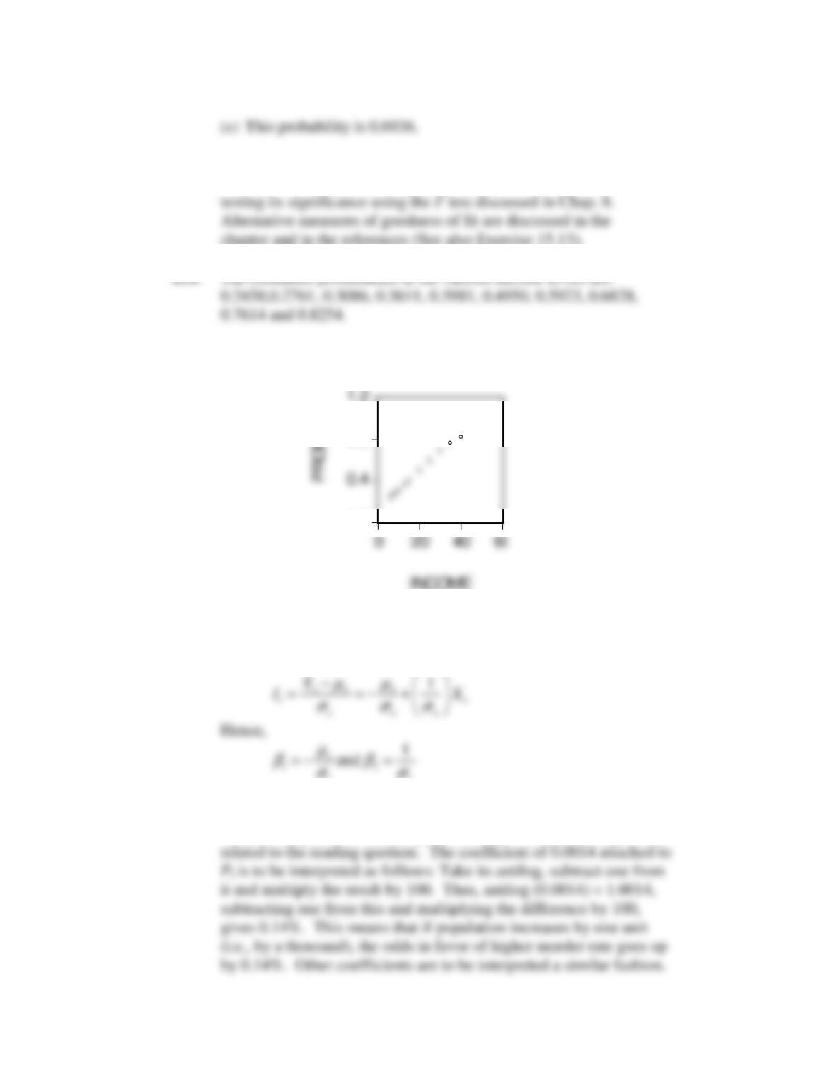
If you plot these probabilities against income, you will almost
obtain an upward-sloping straight line.
15.6 Recall that
1 2
i i
I X
β β
= +
Therefore, the standardized normal variable is:
x x
15.7
(
a
) The log of the odds in favor of higher murder rate is positively
related to population size, the population growth rate but negatively
0.0
0.8
Basic Econometrics, Gujarati and Porter
174
Note:
If you take the coefficients of the regressors at their face
15.8
The estimated coefficients differ little; the main difference comes in
Empirical Exercises
15.9
(
a
) Notice that here the log of the odds ratio is a function of the
(
b
) Taking the antilog of the estimated equation, we obtain
From the preceding expression, we get the expression for probability
of owing a car as follows:
(c) This probability is:
0.3475
0.0625(20000)
Basic Econometrics, Gujarati and Porter
15.11
a) Although the results are not uniform, in several cases the logit
(c) As you can see, if you take all the matriculants, all the
coefficients are highly statistically significant. But this is not the
15.12
(a) To make the error term homoscedastic, the weight should
be the inverse of the standard error of the disturbance term u
i
.
The weight in the present case is:
(b) The weights and the transformed data are as follows:
Probability Weight (
i
w
)
*
i
I Iw
=
*
i i i
X X w
=
0.24 0.086 – 8.113 92.717
0.35 0.140 – 2.708 92.636
0.51 1.991 0.015 10.044
0.66 0.168 2.388 179.124
0.80 0.095 8.820 420.000
(c) The weighted least-squares results are:
Basic Econometrics, Gujarati and Porter
176
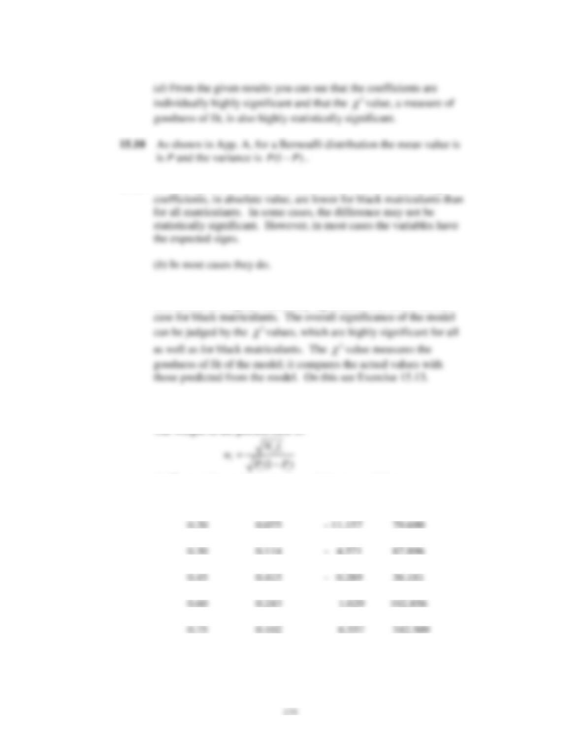
15.13 The
χ
2
test statistic here is 2.3449, whose p value is about 0.97.
15.14 The results of the weighted logit model, relating the probability
of death as a function of the log of the dosage are:
15.15 (a) The results from the LPM model are as follows:
ˆ
2.867 0.003 0.002
Y Q V
= − + +
(b) Although the statistical results look satisfactory, the LPM
15.16
(a) The estimated logit model is:
(b) The estimated probit model is:
Basic Econometrics, Gujarati and Porter
177
(d) We want to find out
15.17
(a) The marital status coefficient is statistically insignificant
for both time periods, so not much can be said about the
(b) The negative estimated coefficient for the minority
15.18
(a) The results of the weighted LPM are:
(b) Given X = 48,
178
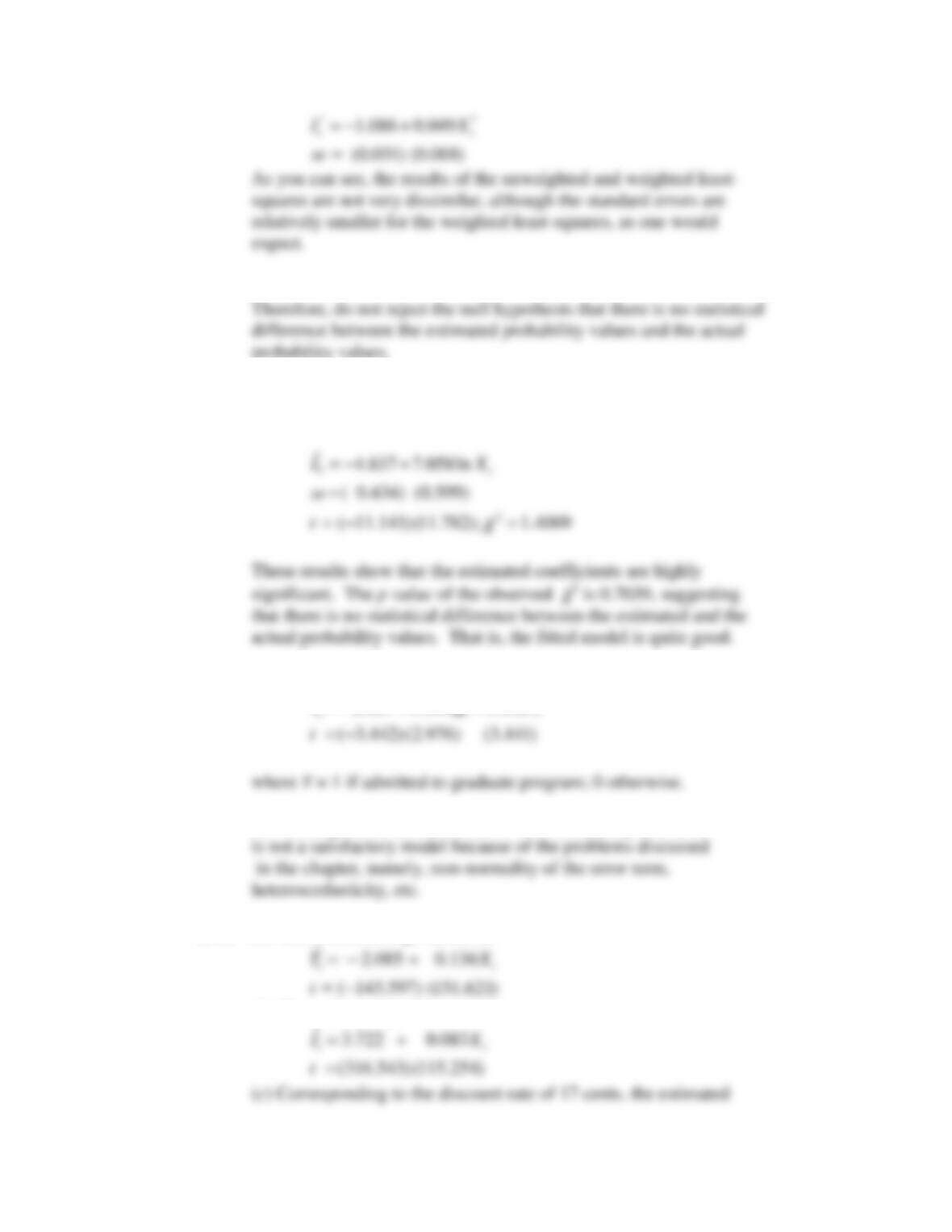
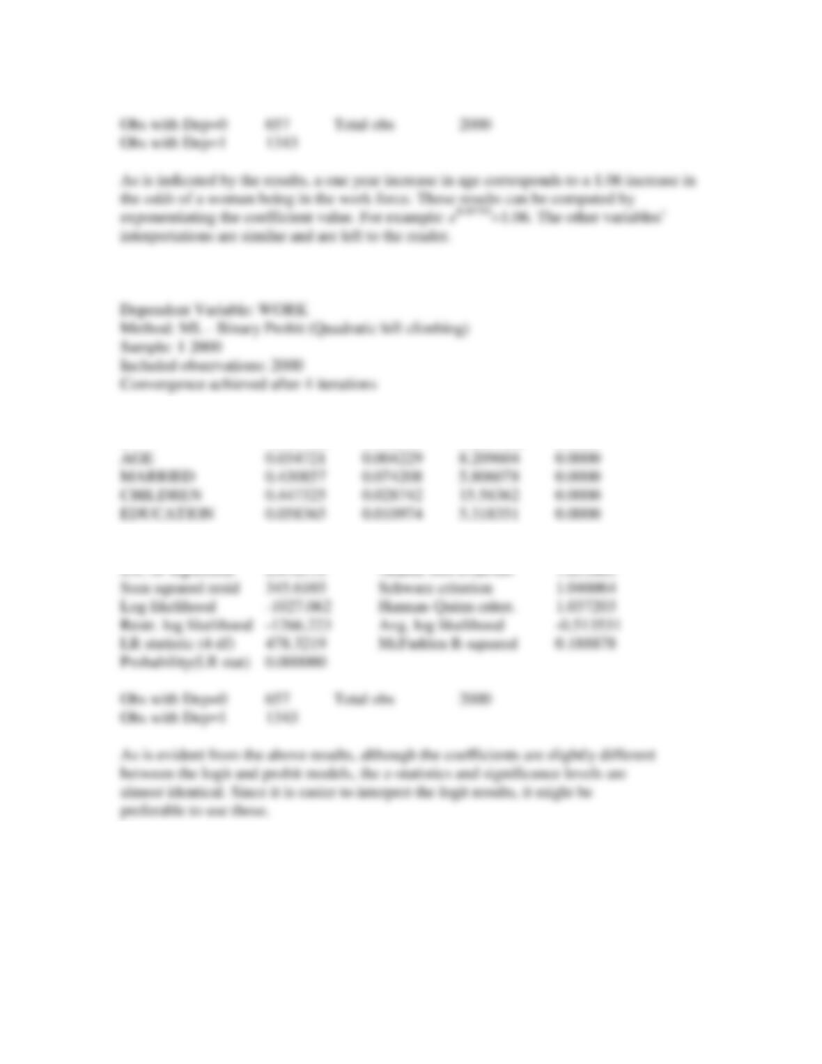
15.19
(a)
Using the data and ‘work’ as the dependent variable, the LPM
results from EViews is as follows:
Dependent Variable: WORK
Method: Least Squares
Sample: 1 2000
Included observations: 2000
Variable Coefficient Std. Error t-Statistic Prob.
C -0.207323 0.054111 -3.831436 0.0001
R-squared 0.202623 Mean dependent var 0.671500
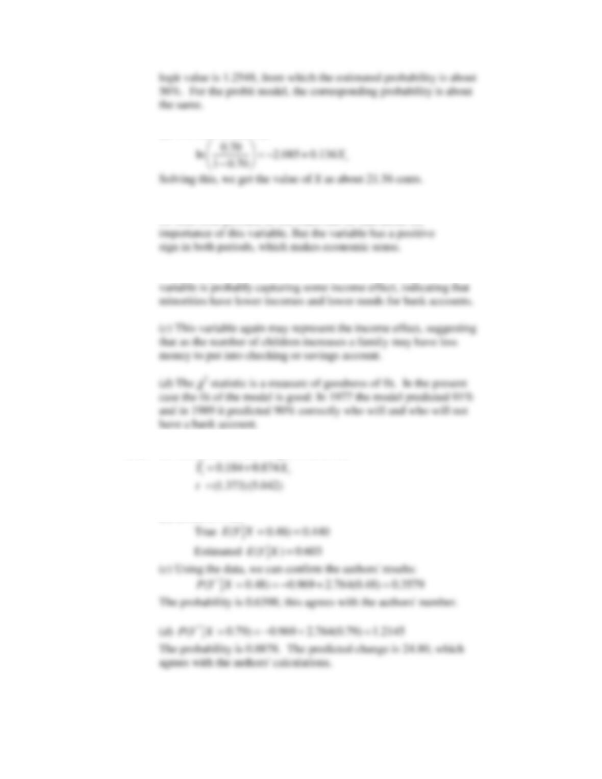
(b)
EViews results for the Logit Model are as follows:
Dependent Variable: WORK
Method: ML – Binary Logit (Quadratic hill climbing)
Sample: 1 2000
Variable Coefficient Std. Error z-Statistic Prob.
C -4.159247 0.332040 -12.52635 0.0000
Mean dependent var 0.671500 S.D. dependent var 0.469785
Basic Econometrics, Gujarati and Porter
179
(c) Results for the probit model are as follows:
Variable Coefficient Std. Error z-Statistic Prob.
C -2.467365 0.192563 -12.81326 0.0000
Mean dependent var 0.671500 S.D. dependent var 0.469785
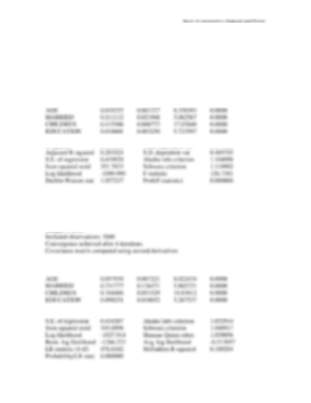
15.20
Logistic Regression results including an interaction term between
Education and Income are as follows:
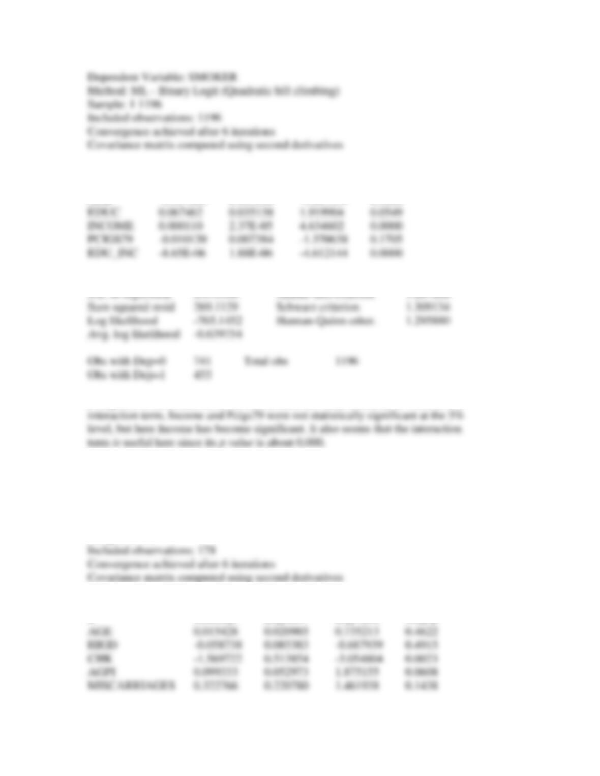
Basic Econometrics, Gujarati and Porter
180
Variable Coefficient Std. Error z-Statistic Prob.
AGE -0.017086 0.003648 -4.683053 0.0000
Mean dependent var 0.380435 S.D. dependent var 0.485697
Compared to the results in Table 15.16, there are some differences. Without the
15.21
EViews results for the logistic model are as follows:
Dependent Variable: CANCER
Method: ML – Binary Logit (Quadratic hill climbing)
Sample: 1 178
Variable Coefficient Std. Error z-Statistic Prob.
C 0.505525 2.224197 0.227284 0.8202
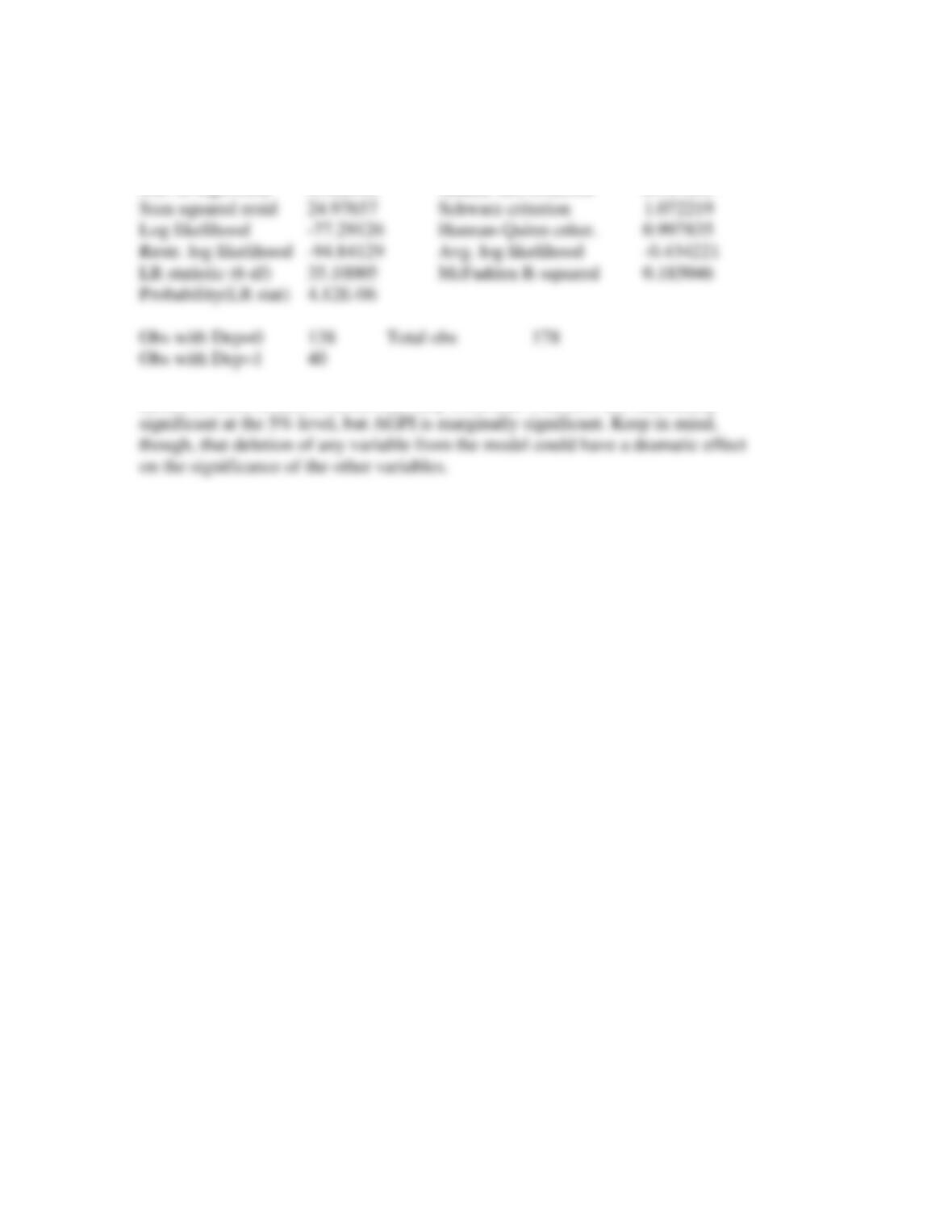
Basic Econometrics, Gujarati and Porter
181
WEIGHT -0.027915 0.009806 -2.846654 0.0044
Mean dependent var 0.224719 S.D. dependent var 0.418575
S.E. of regression 0.382180 Akaike info criterion 0.947093
Based on these results, it seems that only CHK and WEIGHT are statistically