CHAPTER 15
A Dynamic Model of Economic
Fluctuations
Notes to the Instructor
Chapter Summary
Part V of the text presents some advances in macroeconomic theory that clarify our
understanding of the economy. This part of the text begins with Chapter 15, which extends the
analysis of short–run fluctuations to consider the response over time of key macroeconomic
variables. The chapter does this by constructing a dynamic model of aggregate demand and
Comments
The material presented in this chapter is more difficult than the AD–AS, IS–LM models analyzed
in earlier chapters. But because many of the building blocks have already been discussed,
instructors should have a relatively easy time motivating the approach, and students should
readily see the connections to what they have already learned. The model consists of five
equations—a relatively large number for undergraduates to work with—but the discussion
surrounding the model requires only basic algebra. Dynamic solution of the model is done
through simulation exercises, with figures illustrating the time paths of different variables.
Faculty who don’t feel comfortable with going through the algebra of the model’s details can
still use the chapter effectively by relying on the simulation figures to discuss how various
shocks and changes in policy affect the economy over time.
Use of the Dismal Scientist Web Site
Go to the Dismal Scientist Web site and download annual data on the federal funds rate, real
GDP, and the GDP price index over the past 30 years. Compute the trend level of real GDP over
time by graphing it and choosing as endpoints 1979 and 2006 (cyclical peaks). Now construct a
GDP gap series by subtracting your trend GDP from actual GDP. Compute the inflation rate
using the GDP price index. Using the specification of the Taylor rule discussed in Chapter 15,
compute predictions for the federal funds rate over this time period. Now compare your
predictions with the actual federal funds rate. When are they similar and when are they different?
Does the rule fit better after the shift in 1984 to interest–rate targeting and away from monetary–
aggregate targeting by the Federal Reserve? Assess whether your findings suggest that monetary
344 | CHAPTER 15 A Dynamic Model of Economic Fluctuations
Chapter Supplements
This chapter includes the following supplements:
15-2 The Microeconomics of Labor Supply
15-4 Involuntary Unemployment and Overqualification
15-6 Real Business Cycles and Random Walks
15-8 Volatility and Growth
15-9 How Long Is the Long Run? Part Four
15–10 Additional Readings
Lecture Notes | 345
Lecture Notes
Introduction
The chapter builds on the earlier development of the AD–AS, IS–LM models by developing a
dynamic model of aggregate demand and aggregate supply. This model is another way to study
15–1 Elements of the Model
Many of the variables in the model are familiar from previous chapters, but now we will use a
“t” subscript to denote the time period. Thus, total output and national income in period “t” will
be given as Yt and, similarly, in period “t–1” it is given as Yt–1. The model is composed of five
equations, which we describe below.
Output: The Demand for Goods and Services
The demand for goods and services in the economy is determined by:
consumption spending by households, with the response depending on the size of the parameter
α
(a higher interest rate might also appreciate the real exchange rate, dampening net exports).
The demand for goods and services grows with the natural level of output. This feature allows us
to consider long–run economic growth in this model. Finally, the demand shock represents
The Real Interest Rate: The Fisher Equation
We define the real interest as equal to the nominal rate minus expected inflation:
rt = it – Et
π
t+1
which is similar to the Fisher equation. The variable Et
π
t+1 represents the period t expectation of
inflation for period t + 1. Notation and timing reflect the convention of dating variables by when
they are known. Accordingly, the ex ante real interest rate rt and the nominal interest rate it are
Inflation: The Phillips Curve
The model uses a standard Phillips curve, similar to the one derived in Chapter 14:
346 | CHAPTER 15 A Dynamic Model of Economic Fluctuations
Expected Inflation: Adaptive Expectations
Expectations of inflation are formed adaptively, so that last period’s inflation rate is used as the
expectation for inflation in the current period:
Et−1
π
t=
π
t−1.
The Nominal Interest Rate: The Monetary Policy Rule
The last equation of the model is a rule for monetary policy in which the central bank sets a
target for the nominal interest rate based on inflation and output:
it=
π
t+
ρ
+
θπ
(
π
t–
π
t
*)+
θ
YYt−Yt
( )
.
The policy rule assumes that the central bank responds to deviation in inflation from its
target inflation rate
π
t
* and to deviations in output relative to its natural level
Yt
Yt
Yt
. Policy
parameters,
θπ
and
θ
Y, determine how much the central bank responds to these deviations. In the
instrument for the central bank, here the policy instrument is the interest rate. The implicit
assumption here is that the central bank adjusts the money supply as necessary to achieve its
target for the interest rate. Choosing the interest rate as the policy instrument is more realistic as
it closely matches the practice of central banks around the world.
Case Study: The Taylor Rule
funds rate rises by the same amount—0.5 percent. If instead inflation falls below 2 percent or
GDP falls below its natural rate, the federal funds rate falls accordingly. John Taylor’s monetary
rule may be the rule that the Fed implicitly follows in setting policy.
According to the Taylor rule, if inflation and output are low enough, then the nominal
interest rate should be negative. This situation occurred during the financial crisis of 2008–2009.
Lecture Notes | 347
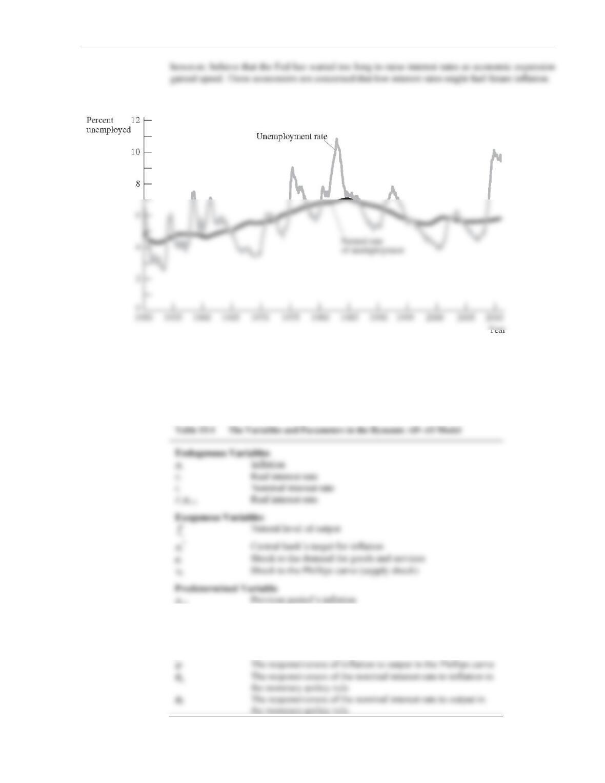
Figure 1: The Unemployment Rate and the Natural Rate of Unemployment in the United States.
15–2 Solving the Model
The five equations presented above determine the paths of the model’s five endogenous
variables: output Yt, the real interest rate rt, inflation πt, expected inflation Et–1πt, and the nominal
interest rate it. Before using the model to analyze the economy’s response to economic shocks,
we first describe the model’s long–run equilibrium.
π
t-1
Parameters
α
The responsiveness of the demand for goods and services to
the real interest rate
ρ
The natural rate of interest
ϕ
The responsiveness of inflation to output in the Phillips curve
π
π
ε
υ
348 | CHAPTER 15 A Dynamic Model of Economic Fluctuations
The Long–Run Equilibrium
Long–run equilibrium for the model is the situation in which there are no shocks and inflation is
constant over time. Applying this to the five equations of the model gives output and the real
The Dynamic Aggregate Supply Curve
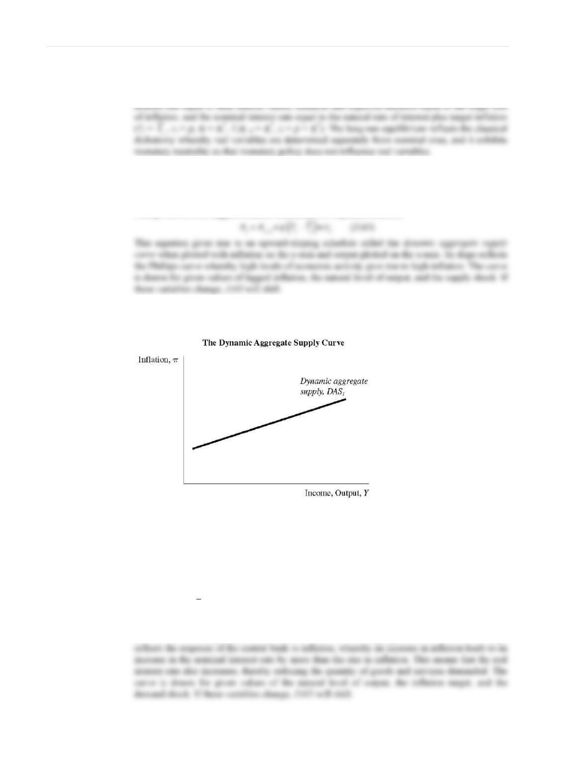
To analyze the economy in the short run, we need to derive two equations that are the analogues
of the AD and AS equations of Chapter 14. The dynamic aggregate supply equation is the
Phillips curve, with lagged inflation substituted for expected inflation:
Figure 2
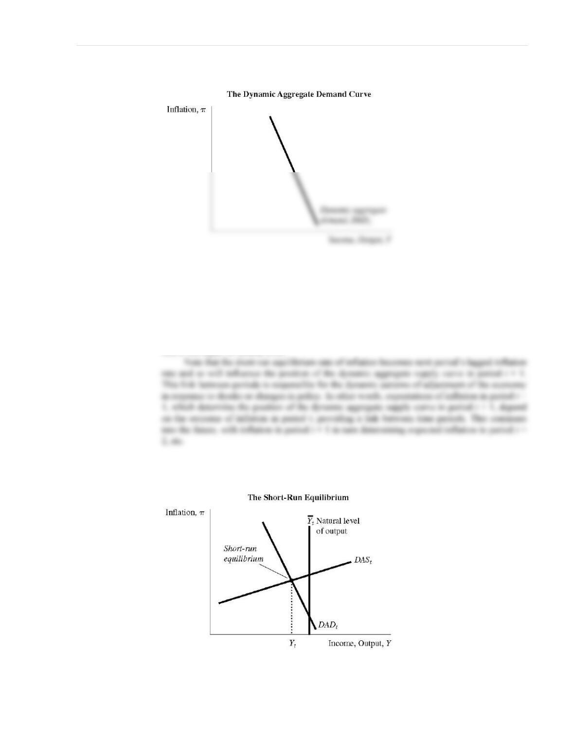
The Dynamic Aggregate Demand Curve
To derive the dynamic aggregate demand curve, start with the demand for goods and services
equation and substitute for the real interest rate using the Fisher equation. Next, eliminate the
nominal interest rate by using the monetary policy equation and substitute for expected inflation
using the equation for inflation expectations. Finally, cancel terms and rearrange the equation to
yield:
Yt=Yt– [
αθ π
/ (1+
αθ
Y)](
π
t–
π
t
*)+[1/ (1+
αθ
Y)]
ε
t.
(DAD)
This equation is represented as a downward–sloping schedule called the dynamic aggregate
demand curve when plotted with inflation on the y–axis and output plotted on the x–axis. Its slope
Lecture Notes | 349
Figure 3
The Short–Run Equilibrium
The intersection of the dynamic aggregate demand curve and the dynamic aggregate supply
curve determines the economy’s short–run equilibrium. These two relationships determine two
endogenous variables (inflation and output in period t), given the five other exogenous (or
predetermined) variables. These are the natural level of output, the target inflation rate, the
demand shock, the supply shock, and the previous period’s inflation rate. The short–run
equilibrium level of output can be less than, equal to, or greater than its natural level. In the long
run, it will equal its natural level.
Figure 4
15–3 Using the Model
We can use the model to assess the effects of change in the exogenous variables. To simplify the
analysis, we assume the economy is initially at its long–run equilibrium.
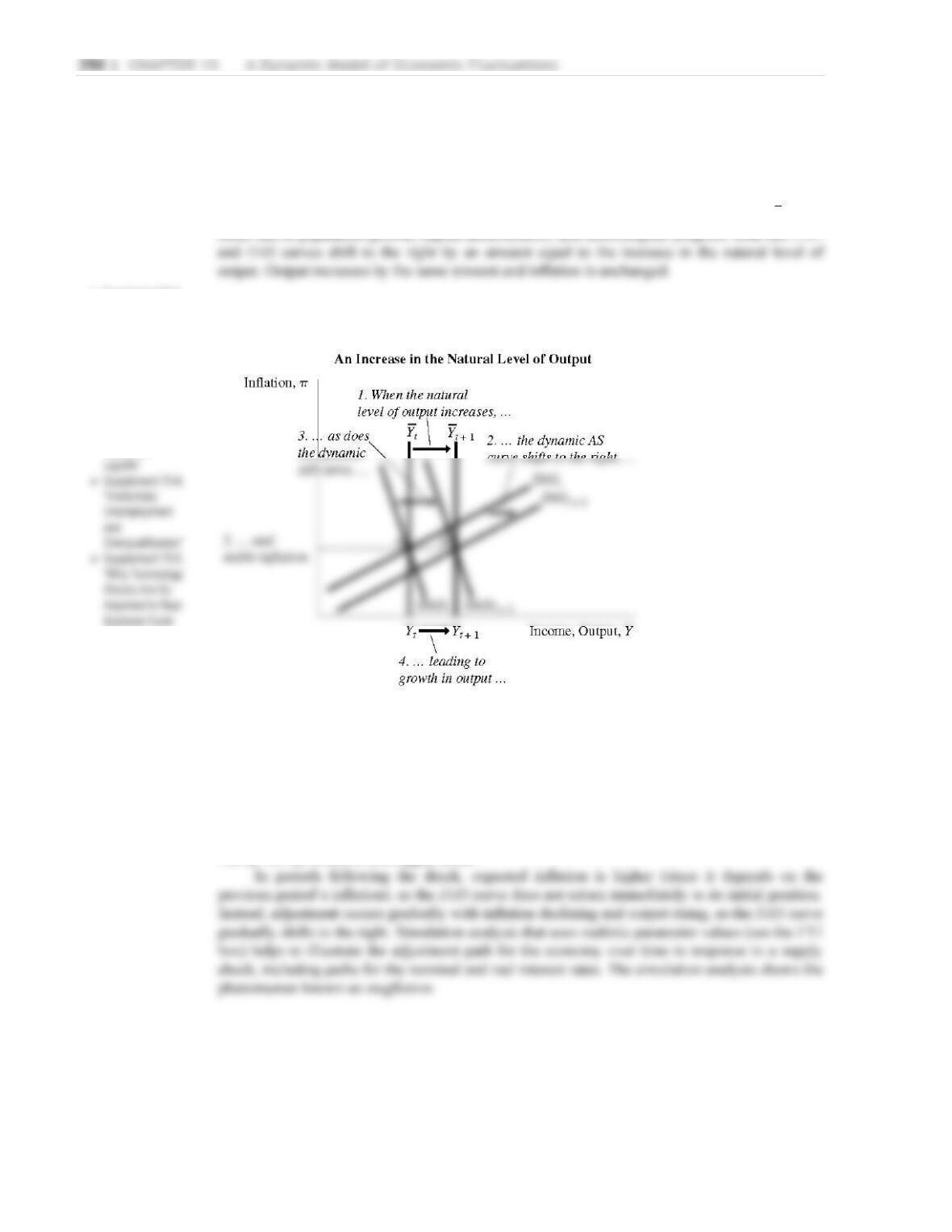
Long–Run Growth
As discussed in Chapters 8 and 9, increases over time in the natural level of output,
Yt
, may
occur due to population growth, capital accumulation, and technological progress. Both the DAD
Figure 5
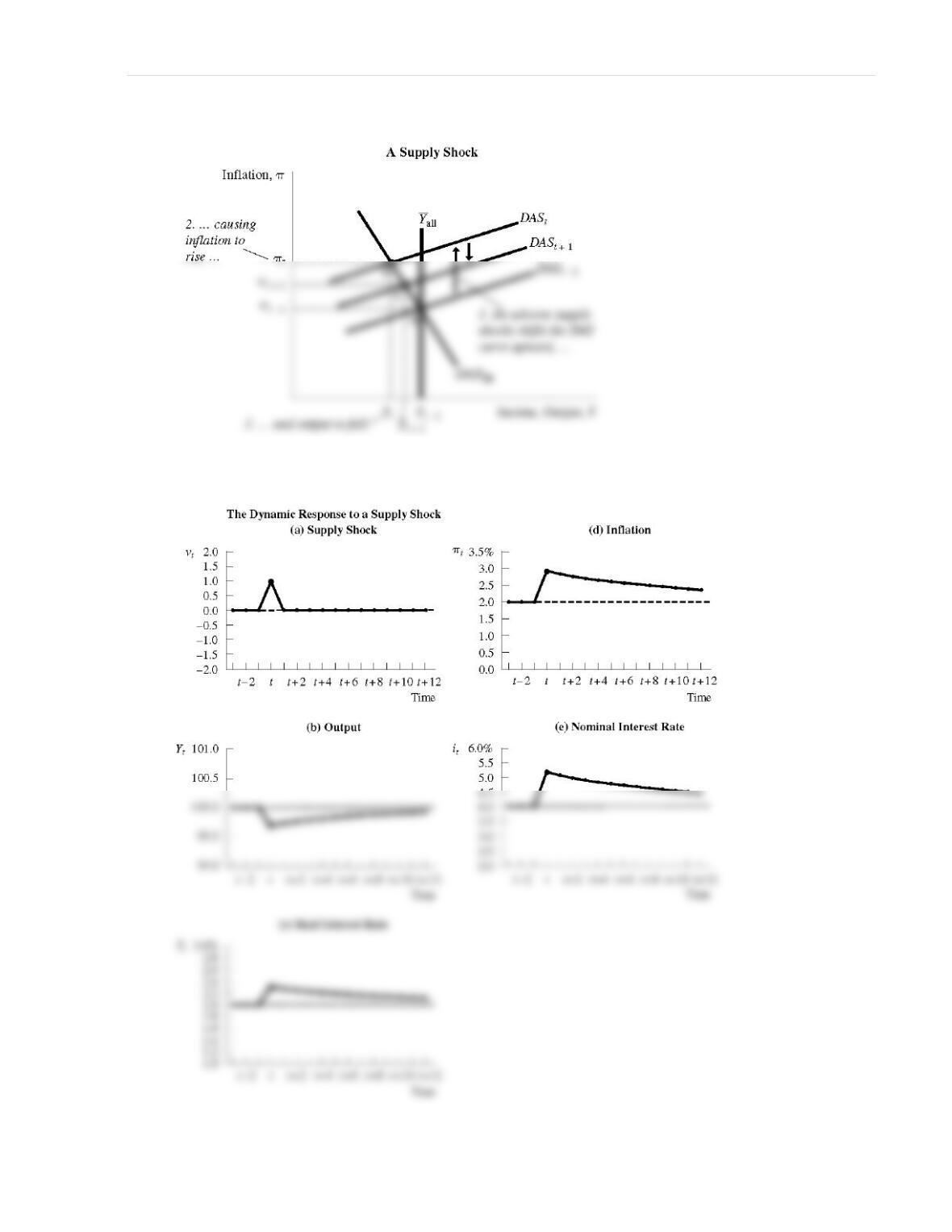
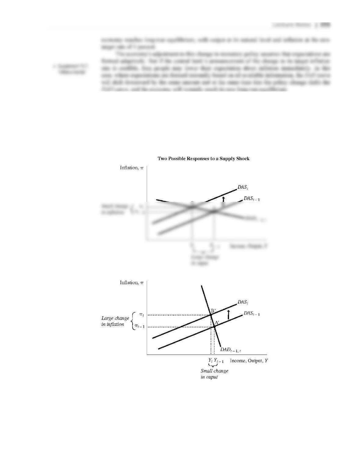
A Shock to Aggregate Supply
Suppose that the aggregate supply shock variable ut increases to 1 percent for one period of time
and then returns to zero. The DAS curve will shift up in period t by exactly the amount of the
shock. The DAD curve will remain unchanged. Inflation rises and output falls in period t. These
effects reflect in part the response of the central bank through its policy rule that leads to higher
nominal and real interest rates, which in turn reduces demand for goods and services and pushes
output below its natural level. Lower output dampens inflationary pressure, so inflation does not
rise by the full extent of the supply shock.
!Supplement 15–1,
“How a Real
Business Cycle
Model Is
Constructed”
!Supplement 15–2,
“The
Microeconomics
of Labor Supply”
!Supplement 15–3,
“Quits and
Models”
!Supplement 15–6,
“Real Business
Cycles and
Random Walks”
Lecture Notes | 351
Figure 6
Figure 7
352 | CHAPTER 15 A Dynamic Model of Economic Fluctuations
FYI: The Numerical Calibration and Simulation
The textbook uses simulation analysis to explore the adjustment of the economy to various
shocks and changes in policies. Each period is best thought of as one year in length. The model
is calibrated using numerical values for the parameters of the model and some of the exogenous
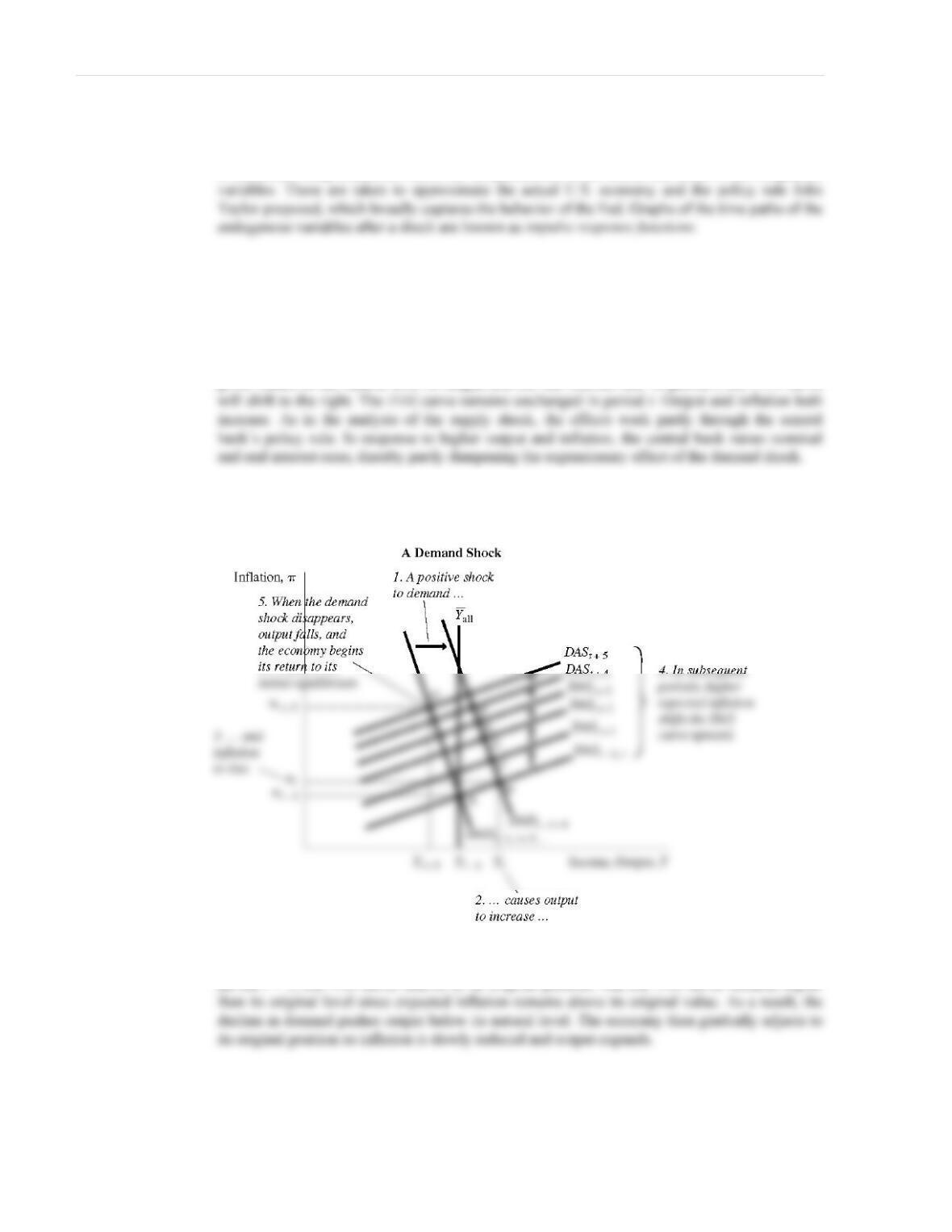
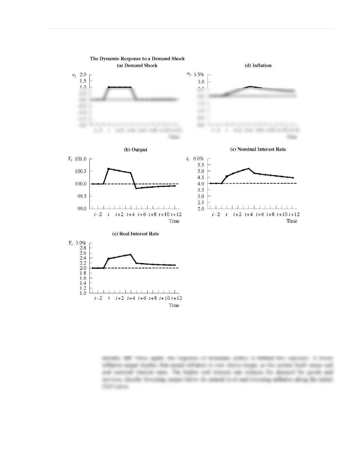
A Shock to Aggregate Demand
Suppose that the aggregate demand shock variable equals one for five periods and then returns to
its normal value of zero. This positive shock might reflect a war that increases government
purchases or a stock–market boom that raises wealth and consumption. More generally, a
demand shock could represent any event that changes the demand for goods and services at
given values of the natural level of output and the real interest rate. In period t, the DAD curve
Figure 8
In subsequent periods, expected inflation is higher, and so the DAS curve shifts upward
continually, reducing output and increasing inflation. When the demand shock disappears in
period t + 5, the DAS curve returns to its original position. But the DAS curve remains higher
Lecture Notes | 353
Figure 9
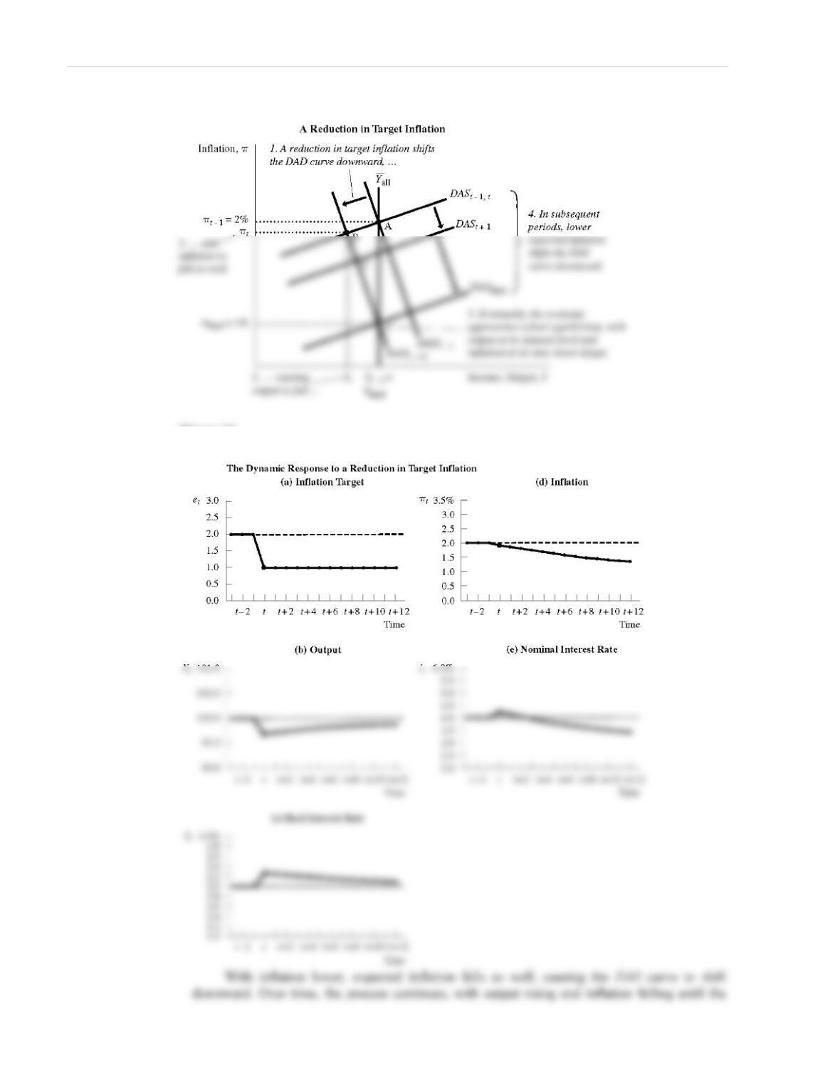
A Shift in Monetary Policy
Suppose that the central bank lowers its target for inflation from 2 percent to 1 percent and keeps
it at the lower value from then on. This will cause the DAD curve to shift to the left (and, to be
exact, downward by one percentage point). Since the target for inflation does not enter the
dynamic aggregate supply equation, the DAS curve does not shift initially. Output and inflation
354 | CHAPTER 15 A Dynamic Model of Economic Fluctuations
Figure 10
Figure 11
15–4 Two Applications: Lessons for Monetary Policy
The model developed in the previous sections can be used to motivate a discussion about the
design of monetary policy. In particular, we can consider how the values of the parameters of the
monetary policy rule influence the effectiveness of monetary policy.
Figure 12
The Tradeoff Between Output Variability and Inflation
Variability
Consider the effect of a supply shock on the economy. As shown earlier, the initial response is
for output to fall below its natural level and inflation to rise above the central bank’s target. But
356 | CHAPTER 15 A Dynamic Model of Economic Fluctuations
the extent to which output declines or inflation rises depends on the slope of the DAD curve.
When the slope is steep, inflation rises relatively more and output declines relatively less,
whereas when the slope is flat, inflation rises relatively less and output declines relatively more.
Because the slope of the DAD curve depends on the parameters of the monetary policy
rule, the central bank can affect the slope by choosing whether to respond more or less strongly
to deviations from target inflation or the natural level of output. In particular, when 8r is large
Case Study: Different Mandates, Different Realities: The Fed
Versus the ECB
The legislation that created the Federal Reserve gave it the dual mandate of stabilizing both
employment and prices, whereas the European Central Bank (ECB) is charged with the primary
objective of maintaining price stability, defined as inflation close to 2 percent over the medium
term. These differences in mandates can be interpreted in our model as being reflected in
different parameters in the monetary policy rule. For the ECB compared to the Fed, more weight
is given to inflation stability and less to output stability. The events of 2008, when oil prices rose
sharply and the world economy headed into recession, support this interpretation: The Fed
lowered interest rates from 5 percent to a range of 0 to 0.25 percent, while the ECB cut interest
rates by much less. In 2011, as the global economy recovered, the ECB began to raise interest
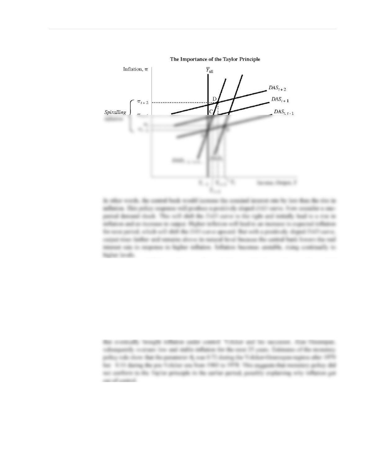
The Taylor Principle
Suppose that the central bank responded to a rise in inflation above its target by cutting the real
interest rate. From the monetary policy equation, this would imply that the parameter 8r is less
than zero:
it=
π
t+
ρ
+
θπ
(
π
t–
π
t
*)+
θ
YYt–Yt
( )
.
Lecture Notes | 357
Figure 13
To prevent inflation getting out of control, the central bank must increase the nominal
interest by more than the rise in inflation (8r must be greater than zero), thereby increasing the
real interest rate, so that the DAD curve is negatively sloped. The requirement that the central
bank respond to inflation by raising the nominal interest more than one–for–one is sometimes
called the Taylor principle, after economist John Taylor, who highlighted it as a key
consideration in the design of monetary policy.
Case Study: What Caused the Great Inflation?
Inflation during the 1970s in the United States reached high levels. Paul Volcker, who was
appointed chairman of the Fed in 1978, instituted a change in monetary policy beginning in 1979
out of control.
15–5 Conclusion: Toward DSGE Models
Advanced courses in macroeconomics develop a class of models known as dynamic, stochastic,
general equilibrium (DSGE) models. The dynamic AD–AS model discussed in this chapter is a
simpler version of these more advanced DSGE models. The model of this chapter illustrates how
the key macroeconomic variables (output, inflation, and real and nominal interest rates) respond
!Supplement 15–9,
“How Long Is the
Long Run?”