
CHAPTER 14
TEACHING NOTES
My preference is to view the fixed and random effects methods of estimation as applying to the
same underlying unobserved effects model. The name “unobserved effect” is neutral to the issue
of whether the time-constant effects should be treated as fixed parameters or random variables.
As a practical matter, the fixed effects and random effects estimates are closer when T is large or
when the variance of the unobserved effect is large relative to the variance of the idiosyncratic
error. I think Example 14.4 is representative of what often happens in applications that apply
pooled OLS, random effects, and fixed effects, at least on the estimates of the marriage and
union wage premiums. The random effects estimates are below pooled OLS and the fixed
effects estimates are below the random effects estimates.
Section 14.3 is new to the fifth edition. I have found that the correlated random effects approach
is useful for several different purposes, including computing a simple test that helps one choose
between random effects and fixed effects estimation.
In the fifth edition I have added a short appendix that describes “cluster robust” inference for
random effects and fixed effects estimation (including correlated random effects). This allows
SOLUTIONS TO PROBLEMS
14.1 First, for each t > 1, Var(uit) = Var(uit – ui,t-1) = Var(uit) + Var(ui,t-1) =
2
2u
, where we use
14.2 (i) The between estimator is just the OLS estimator from the cross-sectional regression of
i
y
on
i
x
(including an intercept). Because we just have a single explanatory variable
i
x
and the
error term is ai +
i
u
i
x
i
u
i
x
i
u
i
x
i
u
i
x
i
x
i
x
i
u
i
x
i
u
i
x
, we have, from Section 5.1,
14.3 (i) E(eit) = E(vit −
i
v
) = E(vit) −
E(
i
v
i
v
) = 0 because E(vit) = 0 for all t.
174
(iii) We must show that E(eiteis) = 0 for t s. Now E(eiteis) = E[(vit −
i
v
)(vis −
i
v
)] =
E(vitvis) −
E(
i
v
vis) −
E(vit
i
v
) +
2E(
2
i
v
) =
2
a
− 2
(
2
a
+
2
u
/T) +
2E(
2
i
v
) =
2
a
− 2
(
2
a
+
2
a
2
u
14.4 (i) Men’s athletics are still the most prominent, although women’s sports, especially
basketball but also gymnastics, softball, and volleyball, are very popular at some universities.
(ii) Tuition could be important: ceteris paribus, higher tuition should mean fewer
applications. Measures of university quality that change over time, such as student/faculty ratios
or faculty grant money, could be important.
i
v
175
(iii) An unobserved effects model is
14.5 (i) For each student we have several measures of performance, typically three or four, the
number of classes taken by a student that have final exams. When we specify an equation for
each standardized final exam score, the errors in the different equations for the same student are
certain to be correlated: students who have more (unobserved) ability tend to do better on all
tests.
(ii) An unobserved effects model is
(iii) Maintaining the assumption that the idiosyncratic error, usc, is uncorrelated with all
explanatory variables, we need the unobserved student heterogeneity, as, to be uncorrelated with
(iv) If SATs and cumGPAs are not sufficient controls for student ability and motivation, as is
14.6 (i) The fully robust standard errors are larger in each case, roughly double for the time-
constant regressors educ, black, and hispan. On the time-varying explanatory variables married
176
and union, the fully robust standard errors are roughly 60 percent larger. The differences are
(ii) On the time constant explanatory variables educ, black, and hispan, the RE standard
errors and the robust standard errors for pooled OLS are roughly the same. (The coefficient
(iii) The robust standard errors for RE are all a little bigger than the usual standard errors.
However, the differences are not huge. The discrepancy for union is the largest: .18 versus .21.
(iv) Because the robust standard errors for RE are all substantially below the corresponding
robust standard errors for POLS, it appears that RE is more efficient than POLS. Of course, we
SOLUTIONS TO COMPUTER EXERCISES
C14.1 (i) This is done in Computer Exercise 13.5(i).
(ii) See Computer Exercise 13.5(ii).
(iii) See Computer Exercise 13.5(iii).
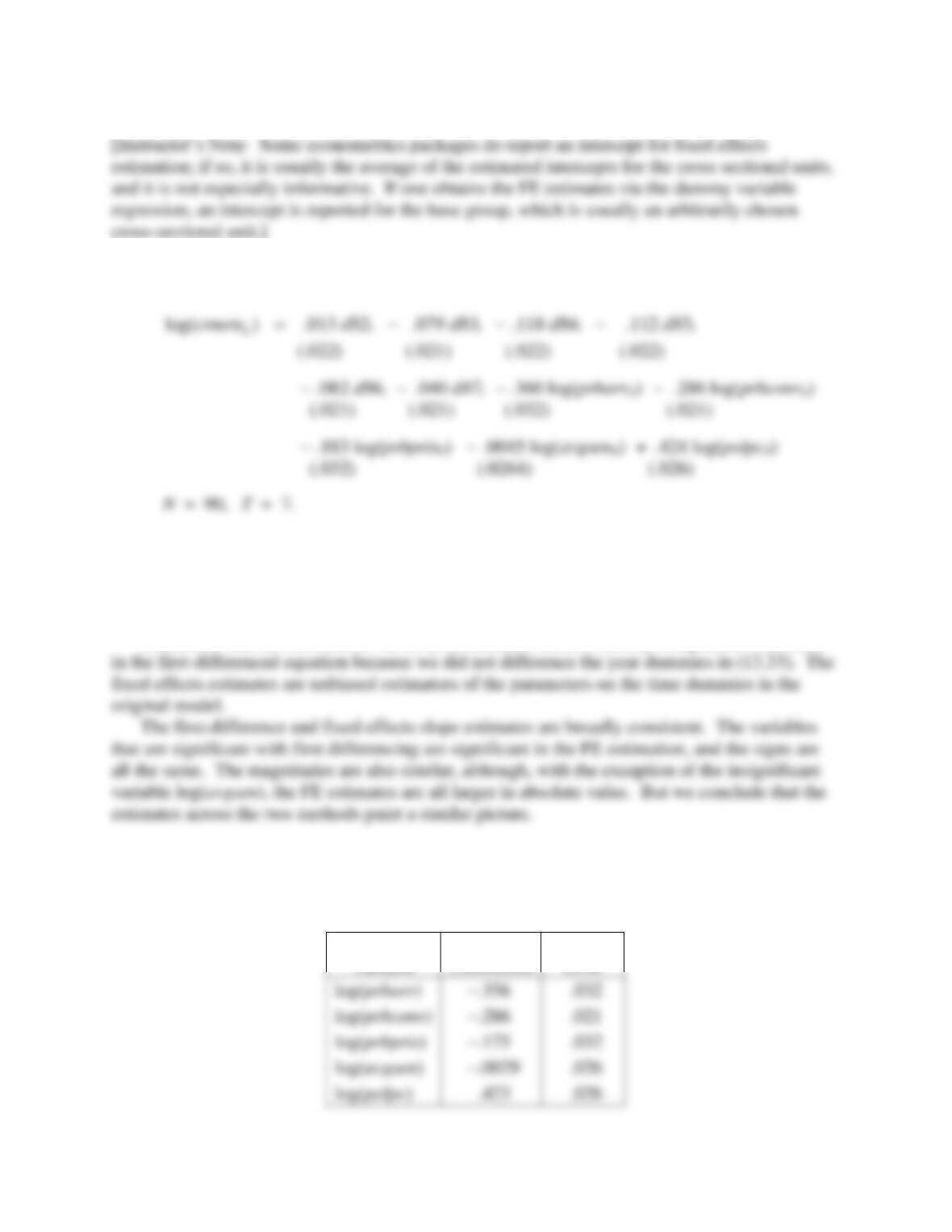
(iv) This is the only new part. The fixed effects estimates, reported in equation form, are
177
C14.2 (i) We report the fixed effects estimates in equation form as
There is no intercept because it gets swept away in the time demeaning. If your econometrics
package reports a constant or intercept, it is choosing one of the cross-sectional units as the base
group, and then the overall intercept is for the base unit in the base year. This overall intercept is
not very informative because, without obtaining each
ˆi
a
, we cannot compare across units.
Remember that the coefficients on the year dummies are not directly comparable with those
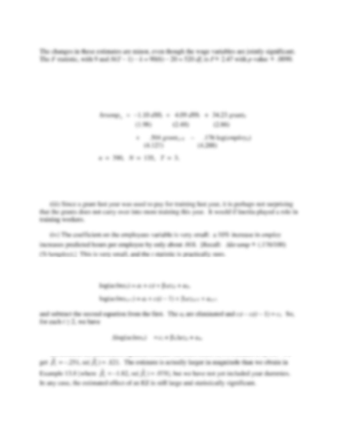
(ii) When the nine log wage variables are added and the equation is estimated by fixed
effects, very little of importance changes on the criminal justice variables. The following table
contains the new estimates and standard errors.
Independent
Standard
178
C14.3 (i) 135 firms are used in the FE estimation. Because there are three years, we would have
a total of 405 observations if each firm had data on all variables for all three years. Instead, due
to missing data, we can use only 390 observations in the FE estimation. The fixed effects
estimates are
(ii) The coefficient on grant means that if a firm received a grant for the current year, it
trained each worker an average of 34.2 hours more than it would have otherwise. This is a
practically large effect, and the t statistic is very large.
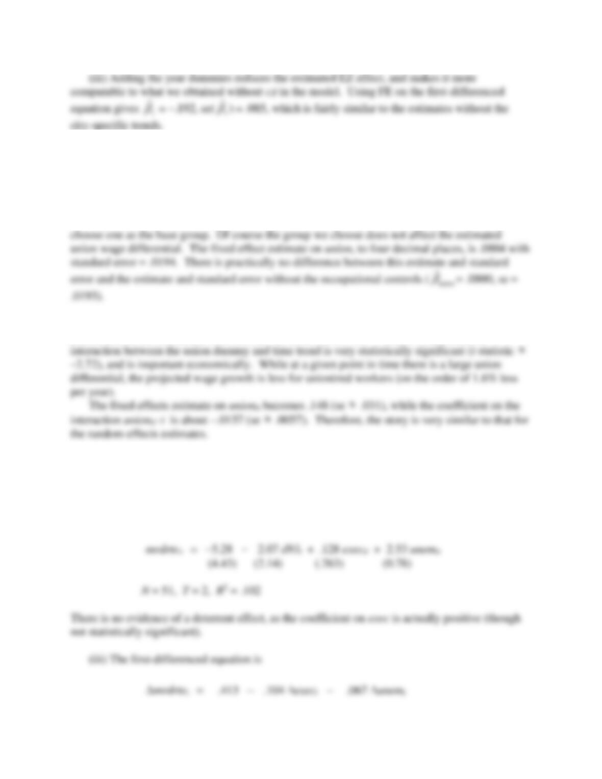
C14.4 (i) Write the equation for times t and t – 1 as
(ii) Because the differenced equation contains the fixed effect ci, we estimate it by FE. We
179
C14.5 (i) Different occupations are unionized at different rates, and wages also differ by
occupation. Therefore, if we omit binary indicators for occupation, the union wage differential
may simply be picking up wage differences across occupations. Because some people change
occupation over the period, we should include these in our analysis.
(ii) Because the nine occupational categories (occ1 through occ9) are exhaustive, we must
C14.6 First, the random effects estimate on unionit becomes .174 (se
.031), while the
coefficient on the interaction term unionit
t is about –.0155 (se
.0057). Therefore, the
C14.7 (i) If there is a deterrent effect then
1 < 0. The sign of
2 is not entirely obvious,
although one possibility is that a better economy means less crime in general, including violent
crime (such as drug dealing) that would lead to fewer murders. This would imply
2 > 0.
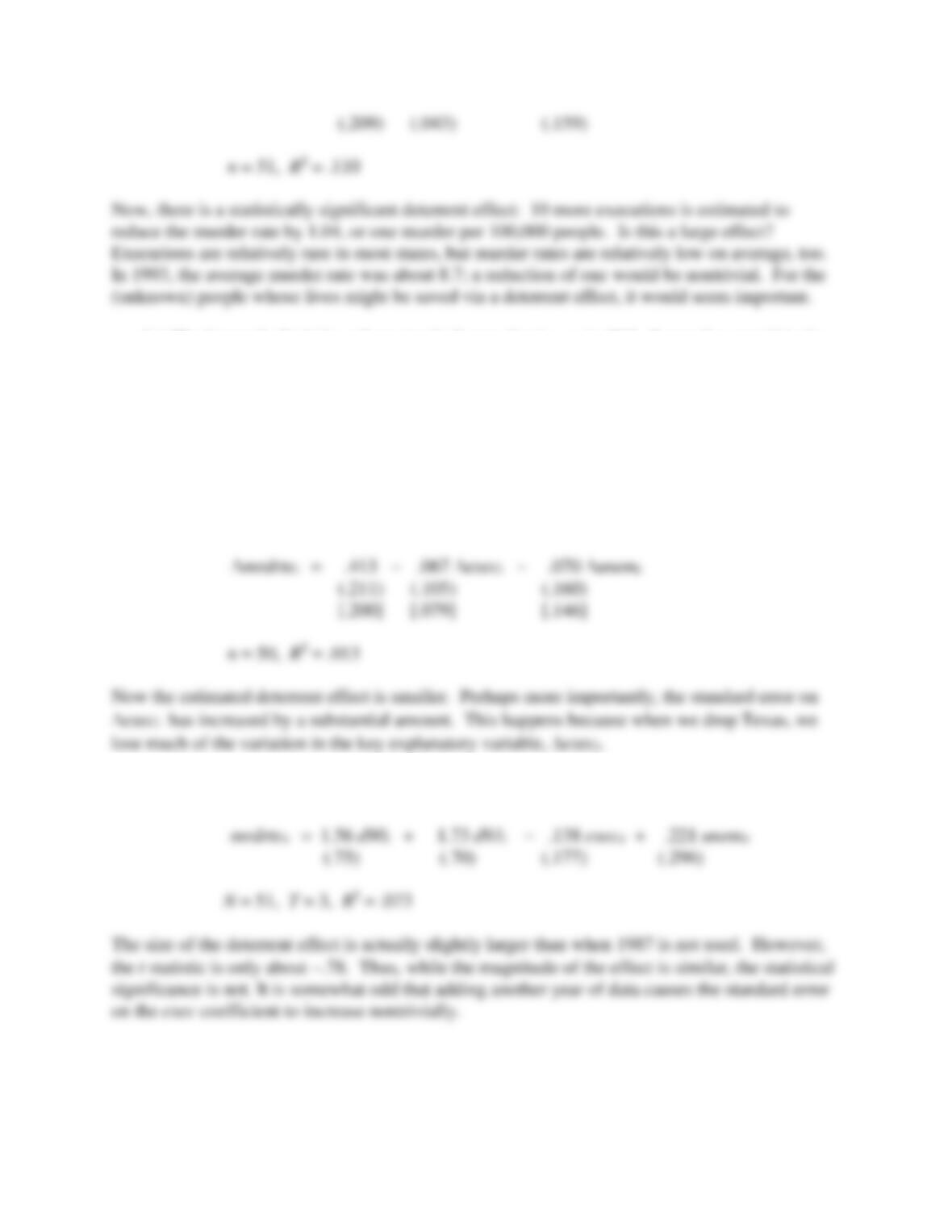
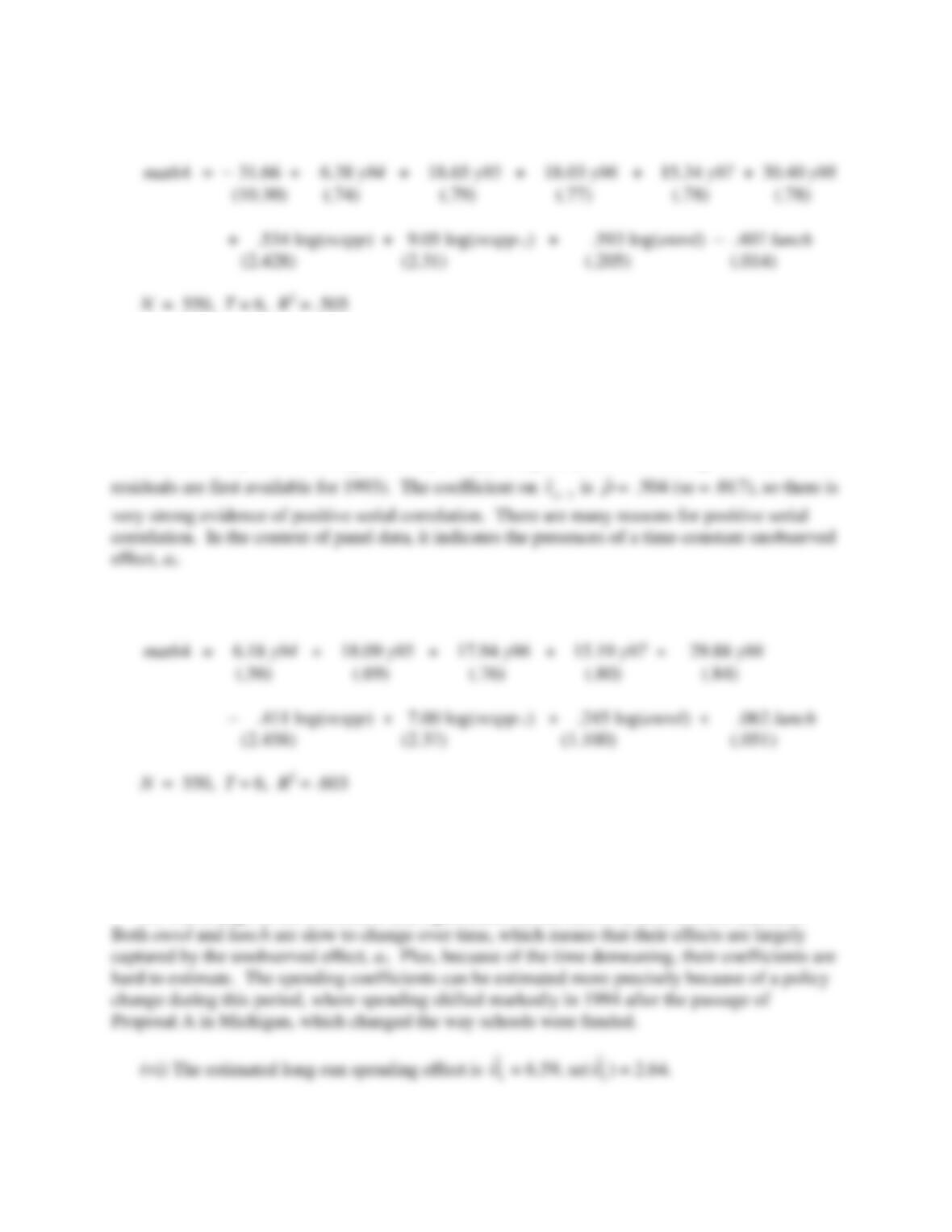
(ii) The pooled OLS estimates using 1990 and 1993 are
180
(iv) The heteroskedasticity-robust standard error for execi is .017. Somewhat surprisingly,
this is well below the nonrobust standard error. If we use the robust standard error, the statistical
evidence for the deterrent effect is quite strong (t −6.1). See also Computer Exercise 13.12.
(v) Texas had by far the largest value of exec, 34. The next highest state was Virginia, with
11. These are three-year totals.
(vi) Without Texas in the estimation, we get the following, with heteroskedasticity-robust
standard errors in []:
(vii) When we apply fixed effects using all three years of data and all states we get
181
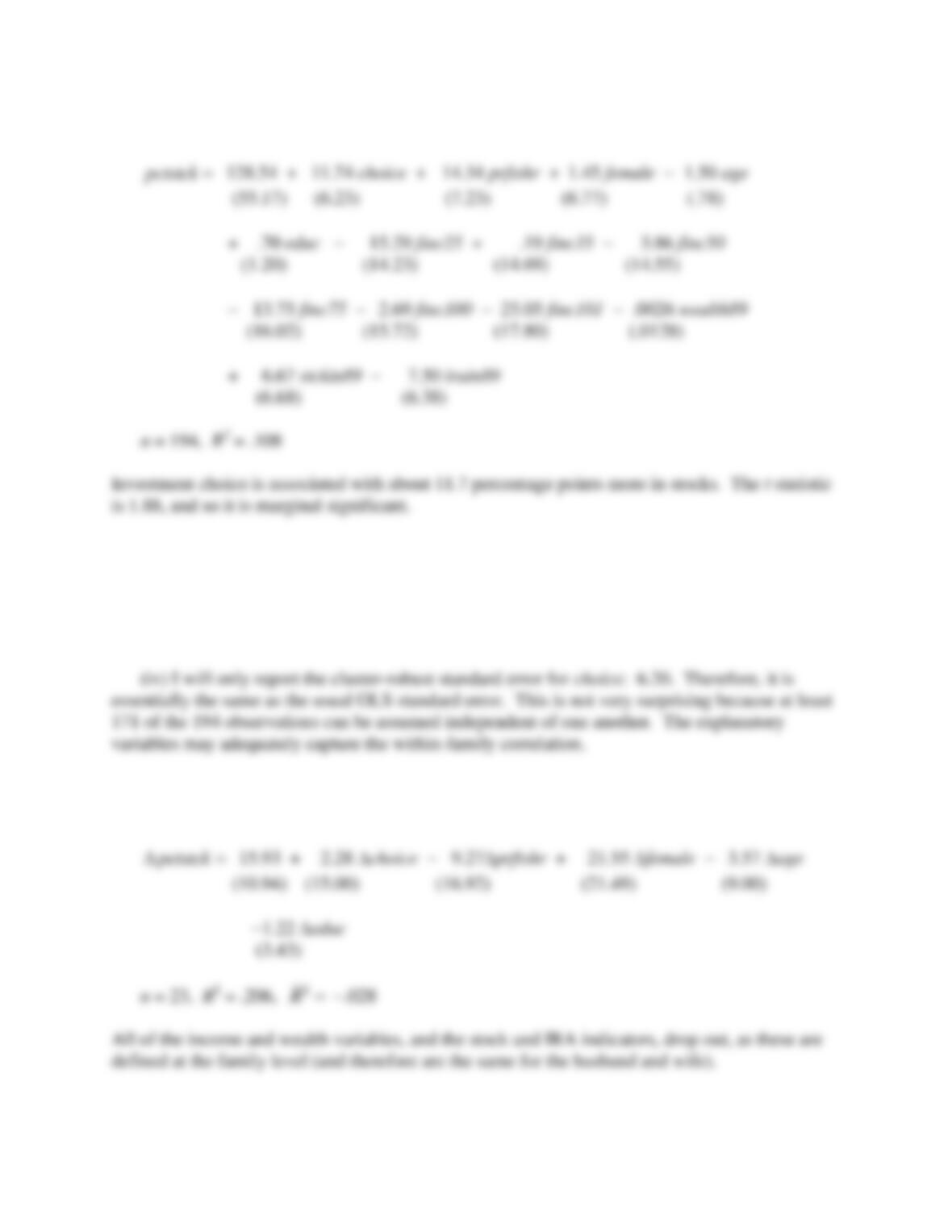
C14.8 (i) The pooled OLS estimates are
(ii) The lunch variable is the percent of students in the district eligible for free or reduced-
price lunches, which is determined by poverty status. Therefore, lunch is effectively a poverty
rate. We see that the district poverty rate has a large impact on the math pass rate: a one
percentage point increase in lunch reduces the pass rate by about .41 percentage points.
(iii) I ran the pooled OLS regression
,1
ˆˆ
on
it i t
vv
−
using the years 1994 through 1998 (since the
(iv) The fixed effects estimates are
The coefficient on the lagged spending variable has gotten somewhat smaller, but its t statistic is
still almost three. Therefore, there is still evidence of a lagged spending effect after controlling
for unobserved district effects.
(v) The change in the coefficient and significance on the lunch variable is most dramatic.
182
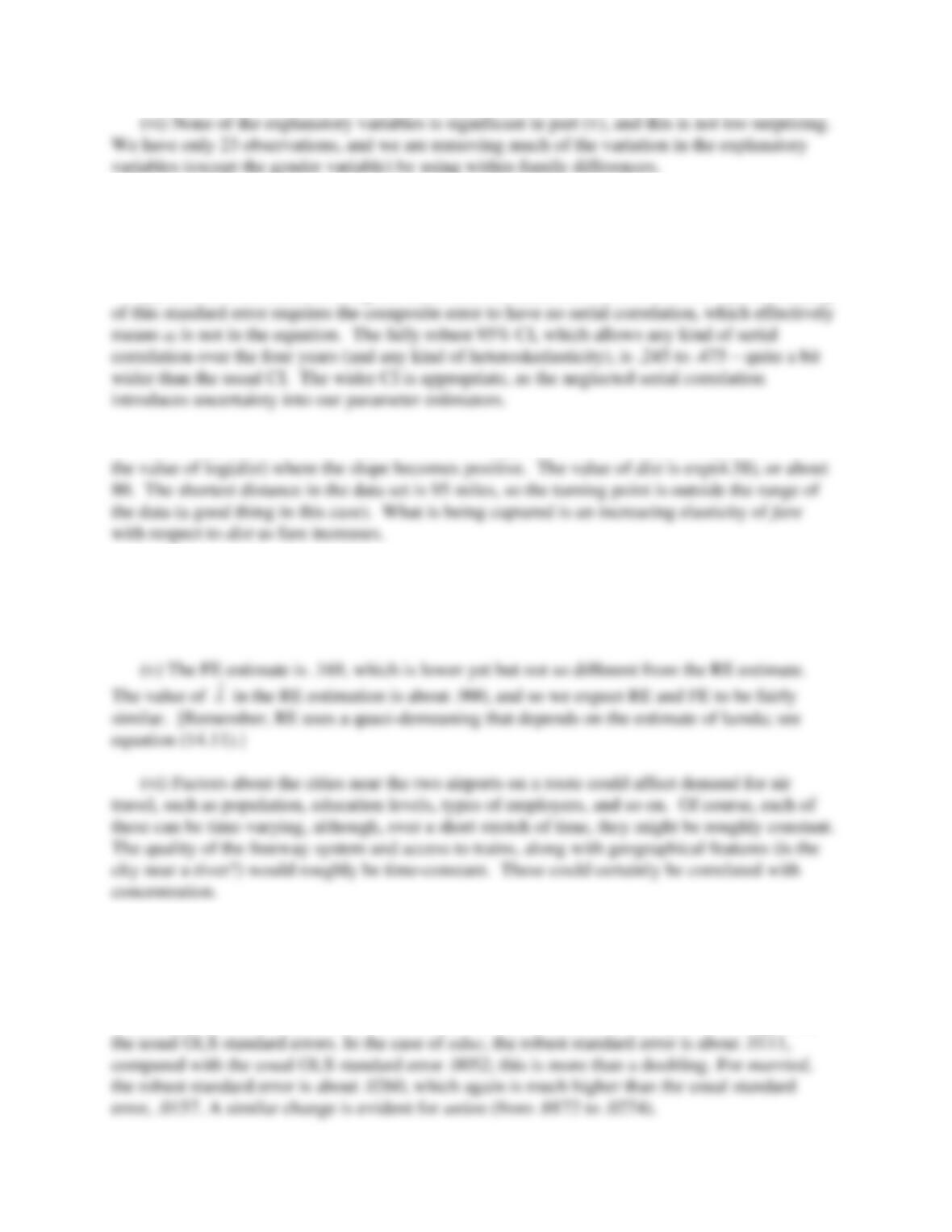
C14.9 (i) The OLS estimates are
(ii) These variables are not very important. The F test for joint significant is 1.03. With 9
and 179 df, this gives p-value = .42. Plus, when these variables are dropped from the regression,
the coefficient on choice only falls to 11.15.
(iii) There are 171 different families in the sample.
(v) There are only 23 families with spouses in the data set. Differencing within these families
gives
183
C14.10 (i) The pooled OLS estimate of
1
is about .360. If
.10concen=
then
.360(.10) .036lfare = =
, which means air fare is estimated to be about 3.6% higher.
(ii) The 95% CI obtained using the usual OLS standard error is .301 to .419. But the validity
(iii) The quadratic has a U-shape, and the turning point is about
.902/[2(.103)] 4.38
. This is
(iv) The RE estimate of
1
is about .209, which is quite a bit smaller than the pooled OLS
estimate. Still, the estimate implies a positive relationship between fare and concentration. The
estimate is very statistically significant, too, with t = 7.88.
(vii) Accounting for an unobserved effect and using fixed effects gives us a positive,
statistically significant relationship. I would go with the FE estimate, .169, which allows for
concentration to be correlated with all time-constant features that affect costs and demand.
C14.11 (i) The robust standard errors on educ, married, and union are all quite a bit larger than
184
(ii) For married, the usual FE standard error is .0183, and the fully robust one is .0210. For
(iii) The relative increase in standard errors when we go from the usual standard error to the
C14.12 (i) The smallest number of schools is one; in fact, 271 of the 537 districts have only one
elementary school in the sample. The largest number of schools in a district is 162. The average
number of schools is about 22.3.
(iv) As we saw in Computer Exercise C9.12, the coefficient on bs is very sensitive to the
(vi) If we just consider estimation with bs .5, pooled OLS gives a small (in absolute
value), statistically insignificant estimate. When we allow for a district fixed effect – which
185
C14.13 (i) The variable totfatrte is the number of traffic fatalities per 100,000 people. Its
(ii) I will not report the entire regression but only discuss the coefficients asked about in the
question. The coefficient on bac08 is about −2.50, which means having a blood alcohol limit of
(iii) The coefficients on the four explanatory variables all change substantially; interestingly,
they are now much closer in magnitude. The coefficients (along with usual t statistic in
parentheses) are:
(iv) The FE estimate of the vehicmilespc is about .00094, so increasing the variable by 1,000
increases the predicted totfatrte variable by about .94. So, if the typical person drove 1,000 miles
more – a pretty large increase – that would lead to about one more fatality per 100,000 people in
the population.

186
(v) I used the “cluster” option in Stata 11 to obtain standard errors valid in the presence of
C14.14 (i) Because there are 1,149 routes – that is, 1,149 different cross-sectional units – there
can be at most 1,149 different values of concenbar. The largest and smallest in the data set are,
respectively, .1862 and .9997. I used the egen command in Stata to create the concenbar values.
(iv) The usual RE t statistic on concenbar in part (ii) is 3.15, with two-sided p-value = .002.
Thus, the RE estimator is strongly rejected (in a statistical sense). Even though the FE and RE
estimates are not very different, we should go with the FE estimate.