CASE STUDY EXTENSION
14–4 Anticipated and Unanticipated Money
Robert Barro pioneered another test of the imperfect–information model.1 An implication of that model is
that anticipated changes in the money supply affect the price level, not output, because anticipated
changes in the money supply increase the expected price level and cause the aggregate supply curve to
shift upward. Unanticipated changes in the money supply affect output.
329
ADVANCED TOPIC
14–5 Is Price Flexibility Stabilizing?
The basic aggregate demand–aggregate supply model suggests that fluctuations in output arise because
shocks cause aggregate demand to fluctuate along an upward–sloping aggregate supply curve. The
aggregate supply curve may slope upward because of price or wage stickiness. This suggests that output
fluctuations will be smaller if prices are more flexible. In particular, if there is a negative shock to
aggregate demand, output will generally fall less, and prices fall more, depending on how steep the
aggregate supply curve is.
There are circumstances, however, in which price flexibility may not make the economy more
stable.11 The basic idea comes from the Fisher equation, which tells us that the real rate of interest equals
the nominal rate minus the expected inflation rate and the fact that aggregate demand depends upon the
real interest rate. Suppose that a fall in aggregate demand leads to a fall in prices, and suppose that falling
prices lead in turn to expectations that prices will fall further in the future. Then falling prices lead to a
decrease in expected inflation and hence an increase in the real interest rate. This leads to a further fall in
aggregate demand. As discussed in Chapter 12, some economists believe that this destabilizing effect of

330
LECTURE SUPPLEMENT
14–6 How Long Is the Long Run? Part Three
Earlier chapters discussed the meaning of the long run in terms of the classical model of Chapter 3 and the
Solow growth model of Chapters 8 and 9. The classical model is a long–run model because prices are
flexible and adjust to ensure that all markets are in equilibrium. The short–run models of Part IV of the
textbook, by contrast, assume some price stickiness, implying that the long run is however long it takes for
prices to be flexible. In the short run, therefore, the aggregate supply curve slopes upward; in the long run,
it is vertical.
ADVANCED TOPIC
14–7 Policy Ineffectiveness
The imperfect–information model of aggregate supply was very influential in the 1970s. One reason is that
it provided a basis for a radical reexamination of the ability of the Federal Reserve to influence the
economy. In particular, two new classical economists, Thomas Sargent and Neil Wallace, put forward a
policy–ineffectiveness argument to the effect that, if people had rational expectations, monetary policy
could not be used to stabilize the economy.11
The basic idea is that people’s expectations about the price level are influenced by their expectations
about the Fed’s actions. Rational individuals understand that if the Fed wishes to stimulate aggregate
demand, it will increase the money supply. They understand further that a higher money supply will raise
where y is output,
y
is the natural rate of output, p is the price level, pe is the expected price level, and we
assume that all variables are in logarithmic terms. Second, we have a simple aggregate demand equation:
y=y+
θ
m−p
( )
+u.
(2)
This equation says that demand depends upon the real money supply (m – p) and a random shock (u). We
suppose for the moment that this shock is observed by everybody, so both the Fed and the private sector
can react to it. The equation is written so that if u = 0, output is at its natural rate when p = m. Finally, we
suppose that the Fed may try to set monetary policy on the basis of the shock to aggregate demand. We
write this as
m = m(u). (3)
The first thing we do is to eliminate p between equations (1) and (2) to get a solution for y. Equation (2)
implies that
p=m–y–y
( )
/
θ
+u/
θ
.
(4)
Substituting (4) into (1) gives
y=y+
α
m−y−y
( )
/
θ
+u/
θ
−pe
( )
,
(5)
332
p
(since this implies y =
y
).
Sargent and Wallace, however, suggested that it wasn’t correct to think about people’s expectations of
the price level as being independent of their expectations of the money supply, for the reasons argued
earlier. They assumed that people had rational expectations. This means that their expectation of the price
is their best possible guess, given the information they have. We write this as pe = E(p), where E( ) is the
symbol for a mathematical expectation. In this case, our first task is to find out what determines people’s
price expectations.
To do so, we go back to equation (4):
p=m–y–y
( )
/
θ
+u/
θ
.
(4)
Using this, we find that
pe=E p
( )
=E m
( )
−E y
( )
−E y
( )
( )
/
θ
+E u
( )
/
θ
(9)
( )
( )
( )
( )
( )
( )
=y.
(10)
This uses the fact that the best guess of a best guess is just the best guess, so the second term equals zero.
The aggregate supply equation, in other words, tells us that, on average, output is at its natural rate. So,
from equations (9) and (10),
pe = E(m) + u/θ. (11)
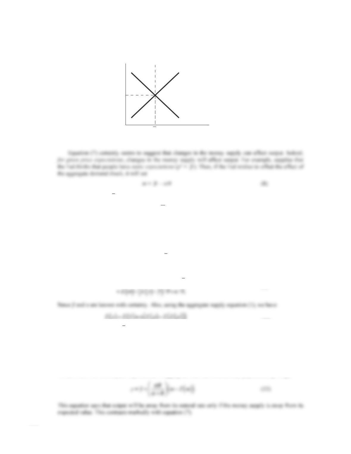
We have now solved for price expectations. Plugging this into the solution for y [equation (7)], we get
p
pe
AS (pe)
AD (m, u)
yy
Figure 1
p
333
What happens if the Fed thinks that people have static expectations, but they actually have rational
expectations? The Fed wishes to stabilize output and so sets the money supply according to the rule
determined in equation (8):
m=p−u/
θ
.
(8)
But people have rational expectations about the Fed and can infer its rule. Thus
E m
( )
=p−u/
θ
=m.
(13)
y=y+
α
/
θ
+
α
( )
( )
u.
(14)
Neither the Fed nor the private sector could do anything about this uncertainty.
Now suppose, however, that the private sector does not observe u, but the Fed does. Then pe = E(m) =
p
. In this case the Fed is able to offset the u shocks by means of monetary policy. When the Fed has an
information advantage, there is room for countercyclical stabilization policy in this model, but not
otherwise.
The policy–ineffectiveness proposition is an example of the Lucas critique, which is discussed in
Chapter 14 of the textbook. The point is that people’s expectations of economic variables are not
independent of the actions of policymakers, since those actions will in general affect the variables. It is
therefore a mistake to suppose that people’s expectations, or more generally their behavior, will remain
unchanged in the face of changes in government policies.
p
334
CASE STUDY EXTENSION
14–8 Did the NAIRU Decline in the 1990s?
As the economy expanded during the 1990s, the unemployment rate fell, dropping below 5 percent in
1997 and reaching a 30–year low of 3.9 percent in 2000. At the same time, inflation remained well
behaved and showed no sign of rising in response to tight labor markets. Many economists believed that
the natural rate of unemployment—or the NAIRU—was about 5 to 6 percent, and so the quiescence of
inflation seemed puzzling when unemployment remained well below this threshold for several years.1
335
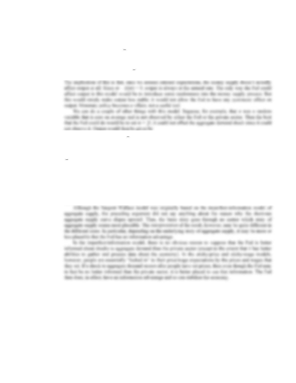
Although favorable supply shocks contributed to the fortuitous combination of low unemployment
and low price inflation, the relationship between unemployment and wage inflation also appears to have
shifted during the 1990s. Accordingly, a more complete explanation requires understanding possible
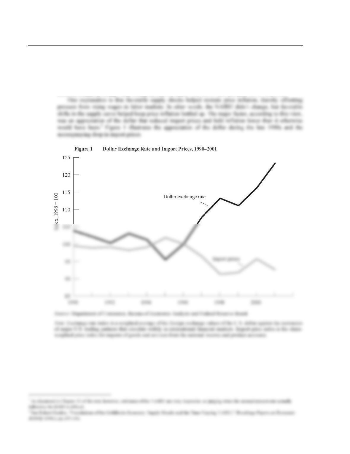
changes in labor markets that may have lowered the NAIRU.3 Here a major factor often highlighted is the
Source: Department of Labor, Bureau of Labor Statistics.
Note: Workers aged 16–24 as a share of labor force aged 16 and over.
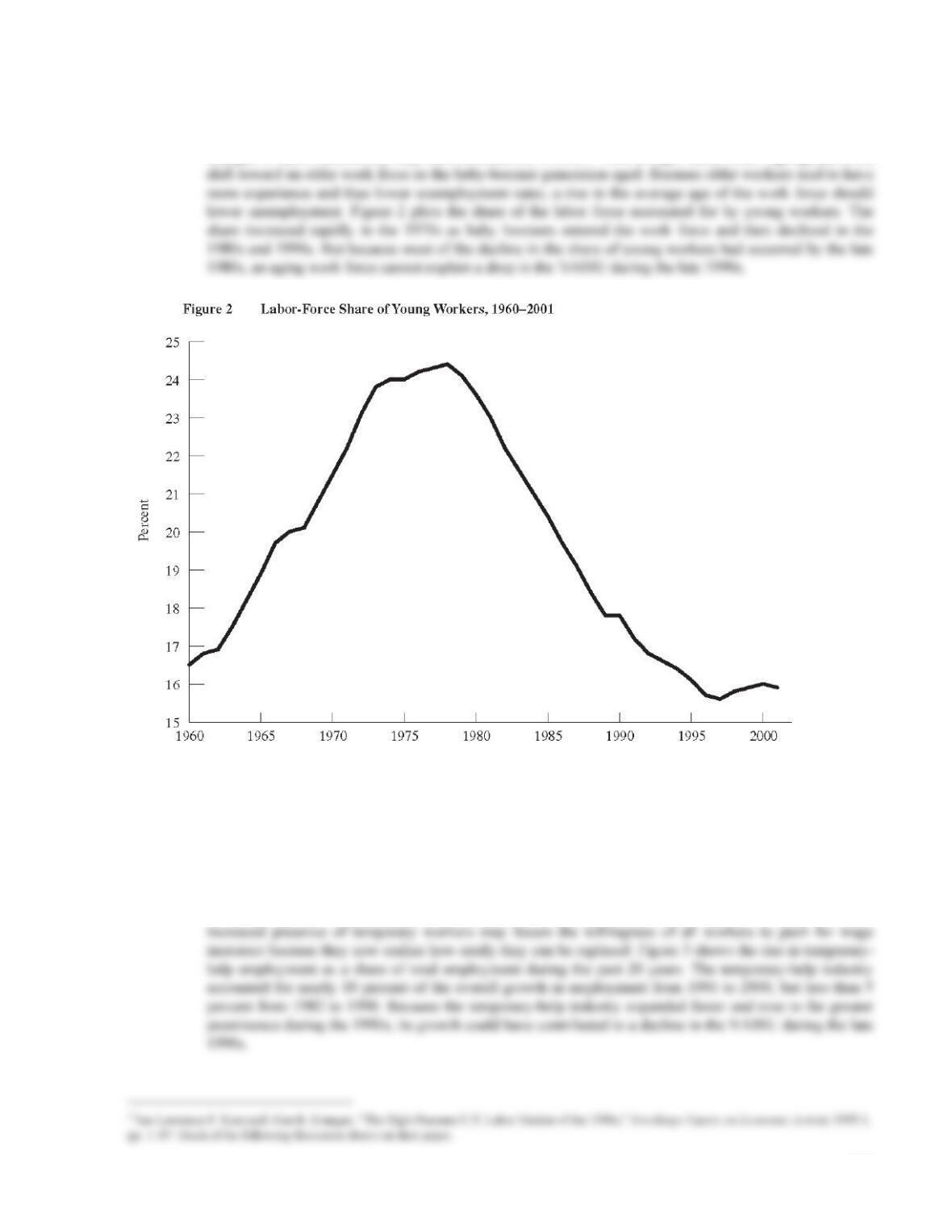
Another factor that could have contributed to a decline in the NAIRU is the recent rapid expansion of
the temporary–help industry. Businesses may be more willing to hire “temps” rather than permanent
employees because the costs associated with hiring permanent employees are greater than those for
temporary help. In particular, temporary–help agencies provide screening and other services, thereby
lowering the cost of hiring and possibly improving the efficiency of job matching. Such improved
efficiency in matching would lead to lower frictional unemployment (see Chapter 6). Furthermore, the
336
Source: Department of Labor, Bureau of Labor Statistics.
Note: Data are employment in the temporary help industry as a share of total nonfarm payroll employment.
Other less important factors that also may have contributed to a decline in the NAIRU include the
continuing erosion of the power of labor unions (see Chapter 7) and the enormous increase in the prison
population since the early 1980s. Because people in prison tend on average to have higher unemployment

CASE STUDY EXTENSION
14–9 Costs of Disinflation
To evaluate the desirability of tight monetary policies aimed at controlling inflation, we really need to
compare the costs of inflation with the costs of disinflation. Analysis of the welfare cost of inflation
suggests that the gain (in reduced “shoe–leather” costs) from reducing the inflation rate by 1 percentage
point is somewhere between $2 billion and $4 billion.1 The textbook suggests that the sacrifice ratio is
about 5, meaning that reducing inflation by 1 percentage point costs about 5 percent of one year’s GDP, or
about $750 billion.
Recession imposes a one–time cost, but the gains from permanently lower inflation persist year after
year. Even without any discounting of the future, however, these estimates suggest it would take literally
hundreds of years before the long–run gain from lower inflation outweighed the cost of the implied
CASE STUDY EXTENSION
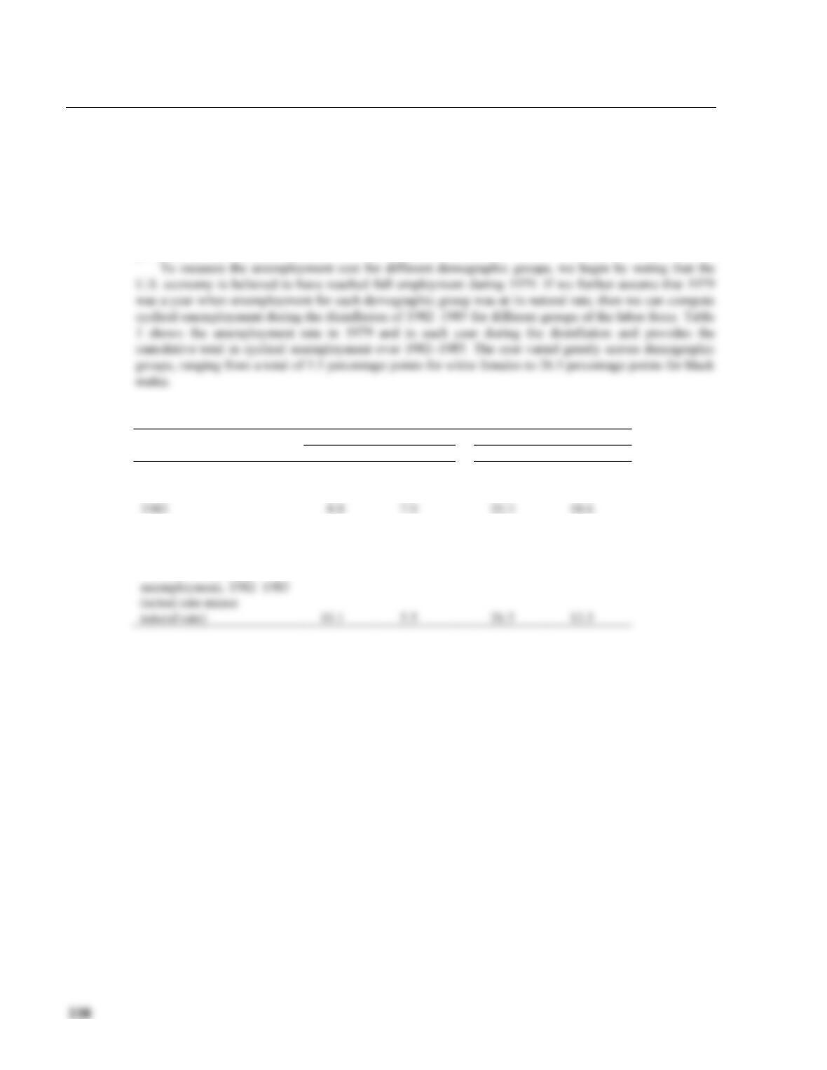
14–10 The Unequal Costs of Disinflation
The sacrifice ratio illustrates the cost of reducing inflation in terms of output lost for the economy as a
whole. During the disinflation from 1982 to 1985, the sacrifice ratio is estimated to have been 3.3
percentage points of GDP lost for each percentage–point reduction in inflation. In terms of unemployment,
the cost was a cumulative total of 10 percentage points of cyclical unemployment (unemployment above
the economy–wide natural rate of 6.0). This cost was somewhat lower than might have been expected
given previous estimates of the sacrifice ratio. Even so, it still varied greatly across different demographic
groups of the labor force.
Table 1 Cyclical Unemployment Rate by Age and Race in the Disinflation of 1982–1985
White
Black
Male
Female
Male
Female
“Natural Rate” (1979 value)
4.5%
5.9%
11.4%
13.3%
1982
8.8
8.3
20.1
17.6
1983
8.8
7.9
20.3
18.6
1984
6.4
6.5
16.4
15.4
1985
6.1
6.4
15.3
14.9
Cumulative cyclical
10.1
5.5
26.5
13.3
ADDITIONAL CASE STUDY
14–11 “The Poincaré Miracle”
The estimates of the sacrifice ratio mentioned in the textbook evidently cannot always be right; otherwise
stopping hyperinflations would cost hundreds of years’ worth of GDP. Bringing a hyperinflation to an end,
as discussed in Chapter 5 of the textbook, involves policymakers’ taking strong measures to balance the
government’s budget and convince the public that policymakers will not again resort to printing money to
1925 and 1926, by about 23 percent.3 Prices were relatively stable for the first three months of 1926 but
grew more rapidly in the following months, rising by over 13 percent between June and July.4 France had
been running budget deficits both during and after World War I, partly in anticipation of paying its deficits
off using reparations from Germany. After Germany was provided with relief from reparations, France had
to either increase its tax revenues or effectively default on its debt by reducing its real value through
Indexation (Cambridge, Mass.: MIT Press, 1983). The following account is based on this article.
3 January–to–January changes in the wholesale price index, calculated from Table 4–1 in Sargent, “Stopping Moderate Inflations.”
4 Not surprisingly, this inflation was accompanied by depreciation of the French franc. See Chapter 6 of the text for the relationship between the
exchange rate and the inflation rate.
5 Sargent, “Stopping Moderate Inflations,” 62.
LECTURE SUPPLEMENT
14–12 Hysteresis and the Long–Run Phillips Curve
Economists used to believe that the Phillips curve reflected a long–run tradeoff between inflation and
unemployment. Policymakers could choose either high inflation and low unemployment or low inflation
and high unemployment. More sophisticated theories of the Phillips curve then incorporated inflation
ADDITIONAL CASE STUDY
14–13 Unemployment in the United Kingdom in the 1980s
Doubts about the natural–rate hypothesis and interest in hysteresis arose largely in response to the
experience in the 1980s of several European countries, especially the United Kingdom. In the 1970s, U.K.
unemployment averaged 3.4 percent, whereas in the 1980s it averaged 9.4 percent. This rise presented a
LECTURE SUPPLEMENT
14–14 Additional Readings
Chapter 14 of the textbook deals with many of the advances in macroeconomics of the last 30 years. Any
short list of readings must be very incomplete. A good place to start is with three of the “Schools Briefs”
published by The Economist: “Paradigm Lost” (November 3, 1990), “Tales of the Expected” (November