313
CHAPTER 14
Aggregate Supply and the Short–
Run Tradeoff Between Inflation
and Unemployment
Notes to the Instructor
Chapter Summary
This chapter summarizes current research on aggregate supply. It is divided into two parts. The
first presents two prominent models of aggregate supply, emphasizing their common conclusion
that output differs from the natural rate if prices differ from expected prices. The models are
Comments
This chapter is one of the textbook’s real strengths. The synthesis of the two models of aggregate
supply brings some unity to an area in macroeconomics in which there is a striking lack of
consensus. From the point of view of explanation (though perhaps not of policy), it is very
helpful to draw out the similarities between the Lucas imperfect–information model and new
Keynesian theories of sticky prices. (Instructors who wish to pursue the policy implications of
these models in more detail could use Supplement 14–7 on policy ineffectiveness.)
Instructors can save time in this chapter by not presenting both models of aggregate supply
and instead emphasizing the supply equation common to all the models. The material in this
chapter requires about two lectures.
Use of the Dismal Scientist Web Site
Go to the Dismal Scientist Web site and download monthly data over the past ten years for the
U.S. consumer price index, both for the overall index and the core index that excludes food and
energy prices. Compute the 12–month inflation rate (i.e., December to December, January to
314 | CHAPTER 14 Aggregate Supply and the Short Run Tradeoff Between Inflation and
Unemployment
Chapter Supplements
This chapter includes the following supplements:
14-2 Real Wages over the Business Cycle
14-4 Anticipated and Unanticipated Money (Case Study)
14-5 Is Price Flexibility Stabilizing?
14-6 How Long Is the Long Run? Part Three
14-8 Did the NAIRU Decline in the 1990s? (Case Study)
14-9 Costs of Disinflation (Case Study)
14–11 “The Poincaré Miracle”
14–13 Unemployment in the United Kingdom in the 1980s
14–14 Additional Readings
Lecture Notes | 315
Lecture Notes
Introduction
The IS–LM model is a useful and versatile model of the economy in the short run when prices
are fixed, and we could spend a long time analyzing its properties. Modern macroeconomics,
though, treats IS–LM as only part of the explanation of short–run fluctuations: It is a theory of
aggregate demand, which must be combined with aggregate supply to obtain a complete picture
of the economy. The reason for this is that the assumption of complete price stickiness, with its
implication of a horizontal short–run aggregate supply curve, is very unsatisfactory. Modern
14–1 The Basic Theory of Aggregate Supply
This chapter introduces an upward–sloping short–run aggregate supply (SRAS) curve. As a result,
changes in aggregate demand will now affect not only output in the short run, but also the price
level. The upward–sloping SRAS curve arises due to “frictions” in the economy that we have thus
(1) the sticky–price model and (2) the imperfect–information model. These models highlight
different “frictions,” and both contain some element of the truth.
The Sticky–Price Model
First, we turn to the sticky–price model. This model is the most widely accepted explanation for
an upward–sloping SRAS curve. The model highlights how firms may sometimes set prices by
long–term contracts with their customers or, in the absence of such contracts, hold prices
constant simply because they don’t want to offend their customers with frequent price changes.
Sticky prices also may result because it is costly to reprint catalogs and price lists or because
nominal wages are sticky (perhaps due to social norms) and firms base their prices on the costs
of production.
316 | CHAPTER 14 Aggregate Supply and the Short Run Tradeoff Between Inflation and
Unemployment
We suppose that a firm’s desired price is denoted by p. This price depends upon two
things. First, the general price level (P): Think of the firm as having a desired real price in mind
and then setting a nominal price based on the overall price level; or, essentially equivalently,
think of the firm’s desired nominal price as depending on both the prices charged by its
competitors and the cost of its inputs. A rise in the general price level causes these to rise and
induces the firm to want a higher price. Second, the firm’s desired price depends upon the level
of demand in the economy. A natural way to model this is to suppose that the firm would like to
set a price equal to the general price level if demand is at its long–run level. If demand is higher,
the firm wants a higher price. We can summarize this as
p = EP.
The actual price level in the economy is the average of these two sets of prices:
P=sEP +1−s
( )
P+a Y −Y
( )
( )
.
We can solve this for P to obtain
P=EP +a1−s
( )
/s
( )
Y−Y
( )
.
This equation tells us, first, that if output is at its natural rate, the actual and expected price levels
correspond. This makes sense. Sticky–price firms simply set their price equal to the expected
price level, whereas if output is at the natural rate, flexible–price firms set their price equal to the
actual price level. These together imply that the actual price level equals the expected price
!Supplement 14-1,
“The Sticky–Wage
Model”
!Supplement 14–2,
“Real Wages
Lecture Notes | 317
An Alternative Theory: The Imperfect–Information Model
The second model of aggregate supply, known as the imperfect–information model, assumes that
markets clear. In other words, prices and wages are free to adjust so that supply equals demand
in goods and labor markets. The market imperfection in this model is a temporary misperception
about prices that causes the short–run aggregate supply curve to differ from the long–run
aggregate supply curve. Robert Lucas developed the model in the early 1970s as a formalization
of the framework sketched by Milton Friedman in his presidential address to the American
Economic Association in 1968.1 For this reason, the short–run aggregate supply curve of this
chapter is sometimes referred to as the Lucas supply curve.
Consider a situation where producers are unable to distinguish perfectly between a shock
to the price of their own output, which would lead them to alter their production, and a shock to
the general price level, the best response to which would be no change in production. Given
some positive price shock, a producer’s best response is somewhere between the two, with the
exact decision on how much extra to produce depending upon how probable he regards each
type of shock to be.
Case Study: International Differences in the Aggregate Supply
Curve
The imperfect–information model is based on the fact that producers may be unable to
distinguish perfectly between shocks to their own price and shocks to the general price level. If,
however, shocks to the general price level predominate, then producers will tend to think that
any given change in their price was probably due to such a shock and will not change output
significantly. The converse is true if shocks to individual prices (real rather than nominal shocks)
predominate. The model thus predicts that in countries where aggregate demand fluctuates a
great deal, the aggregate supply curve will be steep (α will be small). Lucas examined data for
many different countries and found evidence supportive of the theory: Aggregate demand had a
smaller effect on output in countries where prices were highly variable.
!Supplement 14–3,
“The Worker
Misperception
Model””
!Supplement 14–4,
“Anticipated and
Unanticipated
Money”
!Figure 14-1
! Supplement 14–5,
“Is Price Flexibility
Stabilizing?”
! Figure 14-2
! Supplement 14–6,
“How Long Is the
318 | CHAPTER 14 Aggregate Supply and the Short Run Tradeoff Between Inflation and
Unemployment
Implications
The two models of aggregate supply differ in terms of the market friction they emphasize. The
sticky–price model emphasizes that prices may not move to equilibrate supply and demand in the
short run. The imperfect–information model emphasizes the role of information problems as an
explanation of short–run fluctuations. These models together provide reason to believe that
14–2 Inflation, Unemployment, and the Phillips Curve
Deriving the Phillips Curve From the Aggregate Supply Curve
In 1958, the economist A.W. Phillips noted that there was an inverse relationship between the
inflation rate and the unemployment rate. This relationship became known as the Phillips curve
and is specified as
π = Eπ – β(u – un) + ν,
where un is the natural rate of unemployment and ν is a supply shock. To see how this is related
to the SRAS curve, we first write the aggregate supply curve in terms of inflation:
P=EP +1 /
α
( )
Y−Y
( )
P−P
−1=EP −P
−1+1 / 2
( )
Y−Y
( )
⇒
π
=E
π
+1 /
α
( )
Y−Y
( )
FYI: The History of the Modern Phillips Curve
In the early years after Phillips first noted the relationship between inflation and unemployment,
economists thought that it might indicate a simple, stable tradeoff between inflation and
unemployment: Lower unemployment could be achieved only at the cost of higher inflation, and
vice versa. For a time, macroeconomic policy options were often discussed in terms of this hard
choice. Macroeconomists’ understanding of the Phillips curve was greatly increased in the
Lecture Notes | 319
Adaptive Expectations and Inflation Inertia
Modern theories of aggregate supply, as summarized in the Phillips curve, confront a major
difficulty. To use the Phillips curve, we need to have some idea of how people form expectations
of inflation. This is a difficult problem, because expectations are not something we can directly
observe. One possibility is that people look to the recent past; this is known as adaptive
expectations:
Two Causes of Rising and Falling Inflation
The Phillips curve also tells us that inflation will rise if unemployment is below the natural rate
or if there are price or cost shocks. Inflation that arises because of low unemployment, that is, (u
– un) < 0, is called demand–pull inflation. Inflation that arises because of supply shocks is known
as cost–push inflation.
Case Study: Inflation and Unemployment in the United States
U.S. economic history from the 1960s to the 1990s can be summarized in terms of inflation and
unemployment. Broadly speaking, inflation rose and unemployment fell during the 1960s
because of expansionary monetary and fiscal policies. The data for that decade were fairly
consistent with the idea of a stable Phillips curve. In the 1970s, however, unemployment and
inflation both rose, due largely to supply shocks. By the start of the 1980s, high inflation had
been around for a number of years, and inflation expectations were correspondingly high. The
Federal Reserve pursued polices aimed at decreasing inflation, at the cost of a severe recession.
High unemployment and falling oil prices did indeed bring the inflation rate down. In the early
The Short–Run Tradeoff Between Inflation and Unemployment
The Phillips curve does not present policymakers with a permanent tradeoff between inflation
and unemployment; we know that, in the long run, the inflation rate depends upon money
growth and unemployment will be at its natural rate. Policymakers do face such a tradeoff in the
short run, however. By using expansionary monetary and fiscal policies, for example,
policymakers could increase inflation and decrease unemployment in the short run. The theories
of short–run aggregate supply reveal that such a policy would work by increasing prices above
their expected level. If expected inflation changes, the Phillips curve shifts. In the long run,
people revise their price expectations, and there is no tradeoff between inflation and
unemployment.
!Figure 14-3
!Supplement 14–8,
“Did the NAIRU
Decline in the
1990s?”
!Figure 14-4
!Figure 14-5
320 | CHAPTER 14 Aggregate Supply and the Short Run Tradeoff Between Inflation and
Unemployment
FYI: How Precise Are Estimates of the Natural Rate of
Unemployment?
The Phillips curve shows that inflation will tend to rise or fall depending on whether the
unemployment is below or above its natural rate. But measuring the natural rate accurately is
difficult. Estimates of the natural rate—sometimes referred to as the NAIRU (for non–
accelerating inflation rate of unemployment)—are far from precise. One problem is that supply
shocks can cause inflation to rise even when the unemployment rate is high, as we observed in
the mid–1970s. Another problem is that the natural rate may change over time for reasons
discussed in Chapter 6. These include changes in the demographic structure of the workforce,
Disinflation and the Sacrifice Ratio
If policymakers wish to decrease inflation, we know from the long–run analysis that they must
decrease the growth rate of the money supply. In the short run, such a monetary contraction will
cause a recession. It is then natural to ask how costly disinflation is likely to be. The percentage
of a year’s GDP necessary to reduce inflation by 1 percentage point is called the sacrifice ratio.
Although estimates vary widely, a typical value for this number is around 5. In other words, to
reduce the inflation rate by 1 percentage point costs about 5 percent of a year’s GDP.
Rational Expectations and the Possibility of Painless Disinflation
We noted earlier that inflation may have an inertial component: High inflation persists in part
because people expect it. If there was a way to make people revise their expectation of inflation
downward, it would seem possible to reduce inflation without the large costs implied by the
estimates of the sacrifice ratio. To state this another way, the Phillips curve is consistent with
unemployment’s remaining at its natural rate while actual and expected inflation fall together.
If expectations of inflation are rational (people base their forecasts on all available
Case Study: The Sacrifice Ratio in Practice
The Volcker disinflation of the early 1980s permits an estimate of the sacrifice ratio. Between
1982 and 1985, inflation, as measured by the GDP deflator, fell by 6.1 percentage points. Over
the same period, unemployment exceeded the natural rate by a cumulative 10 percentage points.
Using Okun’s law, this translates into 20 percentage points of annual GDP, giving a sacrifice
ratio of 3.3. The relatively low value of this sacrifice ratio may reflect Paul Volcker’s perceived
high credibility. Yet not even Volcker was able to influence inflation expectations sufficiently to
engineer a painless disinflation. Indeed, this reduction in inflation resulted in the most severe
economic downturn at the time since the Great Depression.
Hysteresis and the Challenge to the Natural–Rate Hypothesis
The theory of hysteresis suggests that the natural rate of unemployment may be influenced by
!Table 14-1
!Supplement 14–9,
“Costs of
Disinflation”
!Supplement 14–10,
“The Unequal
Costs of
Disinflation”
!Supplement 14–11,
“‘The Poincaré
Miracle’”
Lecture Notes | 321
the history of the unemployment rate itself. Recessions may not only increase unemployment
above the natural rate in the short run but may also have the effect of increasing the long–run
natural rate itself. In such a setting, it is not clear that the term natural rate has much meaning
anymore.
Recessions can affect the natural rate by reducing workers’ human capital. It is possible
that unemployed workers lose skills, making them less productive. Similarly, recessions might
affect the mix of insiders and outsiders in the economy, as insider workers are laid off and
become outsiders. Both arguments suggest that a temporary recession permanently increases the
14–3 Conclusion
Theories of aggregate supply are controversial, and not all economists agree with the ideas
presented in this chapter. Ten years from now, some of these ideas will probably be better
integrated into our overall understanding of the economy, while others may have been discarded
as a result of theoretical advances or because they have been refuted by economic events. New
Appendix: The Mother of All Models
This appendix illustrates how the classical theory of Part II of the text and the business–cycle
theory of Part IV of the text can be viewed as special cases of a larger framework. The general
framework is given by seven equations:
Y = C(Y – T) + I(r) + G + NX(ε) IS: goods market equilibrium
M/P = L(i, Y) LM: money market equilibrium
NX(ε) = CF(r – r*) Foreign exchange market equilibrium
i = r + Eπ Relationship between real and nominal interest rates
!Supplement 14–12,
“Hysteresis and the
Long Run Phillips
Curve”
322 | CHAPTER 14 Aggregate Supply and the Short Run Tradeoff Between Inflation and
Unemployment
so that they are always correct, the quantity equation holds (velocity is constant), and there are
no international capital flows (the economy is closed). The level of output will always be at its
natural rate, the real interest rate will adjust to clear the goods market (i.e., to ensure that
investment equals saving), the price level will be determined directly by the money supply, and
the nominal interest rate will adjust one–for–one with expected inflation. The classical dichotomy
holds.
Another example is the basic IS–LM model for a closed economy presented in Chapters 11
and 12. Here, we assume α is infinite and that CF(r – r*) = 0. In other words, the aggregate
supply curve is horizontal and the economy is closed. In this case, for any given level of
!Figure 14-6
LECTURE SUPPLEMENT
14–1 The Sticky–Wage Model
Another explanation for why the aggregate supply curve slopes upward in the short run relies on sticky
nominal wages. The sticky–wage model focuses attention on wage–setting agreements made by firms and
workers.
Observation of the economy tells us that in unionized industries, nominal wages are usually set in
the firm and the workers also form an expectation of the general price level. They ultimately set the
nominal wage using the formula
W = ω × EP,
where ω is the target real wage.
Since the wage is set in advance in a contract, the actual price level may turn out to be different from
( )
( )
( )
( )
Notice first that if EP = P, then W/P = ω, so Ld (W/P) = L and Y =
Y
. Now suppose that the actual price
turns out to be higher than was anticipated. Then the actual real wage is lower than anticipated. Labor is
cheaper, so firms will employ more workers and output will increase. Exactly the opposite is true if the
actual price is lower than expected. Firms are getting less revenue for their output than they anticipated, so
they cut back production. We can illustrate this in terms of the labor market. An alternative representation
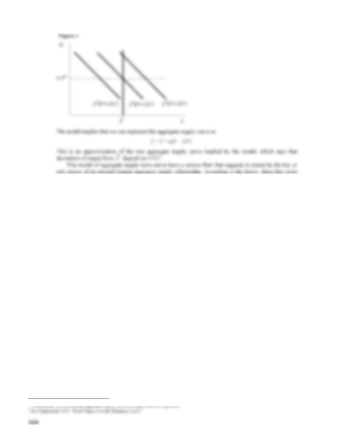
labor and produce more output when the real wage is low. If this were the explanation of business–cycle
fluctuations, then we should expect to see a countercyclical real wage (that is, a real wage that rises when
output falls, and vice versa). In reality, the real wage seems to be acyclical or slightly procyclical,
although measurement problems preclude a definitive conclusion.2
1 Alternatively, think about the aggregate supply curve as being written in log terms.
LECTURE SUPPLEMENT
14–2 Real Wages over the Business Cycle
A paper on the behavior of real wages by Robert Barsky and Gary Solon starts by quoting three studies, all
published in the 1980s, which concluded that real wages were, in turn, acyclical, procyclical, and
countercyclical.1 Although the issue has clearly not yet been fully resolved, Barsky and Solon clarify
possible sources of these different findings.
wages when inflation is countercyclical, and vice versa. This is borne out by the data.
Finally, we can note that theories of implicit contracts (see Supplement 7–8) suggest that the
combination of real wage and employment that we observe at any moment might not really represent the
intersection of a labor supply curve and a labor demand curve. Interpretations of procyclicality as arising
from labor demand shifts along a fixed supply curve, or countercyclicality as arising from labor supply
LECTURE SUPPLEMENT
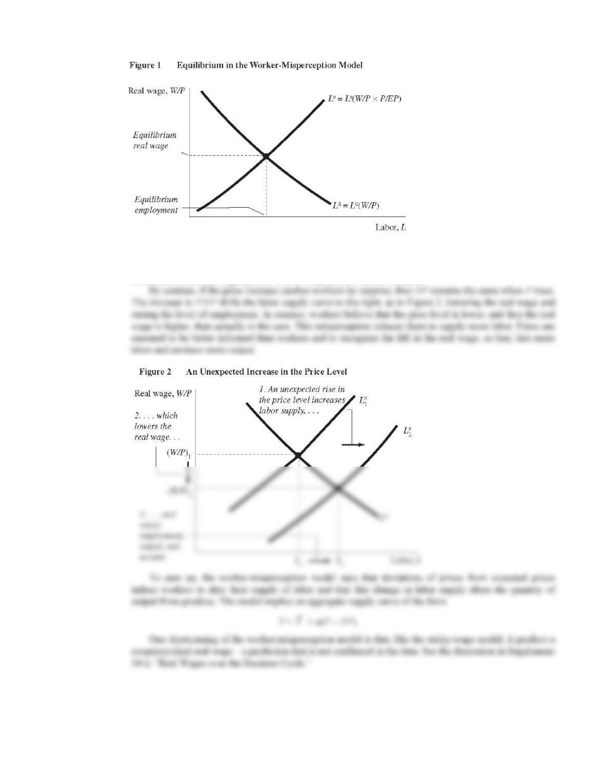
14–3 The Worker–Misperception Model
The worker–misperception model is similar to the imperfect–information model presented in the text in that
both models rely on temporary misperceptions about prices to generate an upward–sloping short–run
aggregate supply curve, while maintaining price and wage flexibility. A main difference between these
models is that the imperfect–information model assumes that all people in the economy are equally
the expected real wage, W/Pe. The expected real wage can be rewritten as:
W/Pe = W/P × P/EP
which shows how the expected real wage is related to the degree of misperception about the price level.
When P/Pe is greater than one, workers will believe, incorrectly, that their real wage is higher than it
actually is, and when P/EP is less than one, workers will mistakenly believe that their real wage is lower
327
Whenever the price level P rises, the reaction of the economy depends on whether workers anticipate
the change. If they do, then EP rises proportionately with P. In this case, workers’ perceptions are
accurate, and neither labor supply nor labor demand changes. The nominal wage rises by the same amount
as prices, and the real wage and the level of employment remain the same.