Economics Chapter 14 Homework Equating The First Derivative Zero Produces 12

Chapter 14

Maximum Likelihood Estimation

◼ Exercises

1. The density of the maximum is

n[z/]n − 1(1/), 0  z  .

2. The log likelihood is lnL = −nln − (1/)

=

1.

n

i

ix

=

1

n

i

ix

The maximum likelihood estimator is obtained as

3. The log likelihood is lnL = nln − ( + )

=

1

n

i

iy

+ ln

=

1

n

i

ix

+

=

1ln

n

ii

ixy

−

=

1ln( !).

n

i

ix

The first and second derivatives are lnL/ = n/

=

−1

n

i

iy

=

1

n

i

iy

=

1

n

i

ix

Therefore, the maximum likelihood estimators are



ˆML

= 1/

y

and



ˆ

=

/,xy

and the asymptotic

Chapter 14 Maximum Likelihood Estimation 115

Thus, x has a geometric distribution with parameter  = /( + ). (This is the distribution of the

number of tries until the first success of independent trials each with success probability 1 − .)

Its asymptotic variance is obtained using the variance of a nonlinear function

A solution is obtained by first noting that at the solution, (1 − )/ =

x

= 1/ − 1. The solution for  is,

thus,



ˆ

= 1/(1 +

x

). Of course, this is what we found in part (b), which makes sense.

Therefore, the maximum likelihood estimator of  is (1 +

x

)/

y

and the asymptotic variance,

conditional on the xs is Asy.Var.

ˆ







= (2/n)/(1 +

x

).

116 Greene • Econometric Analysis, Seventh Edition

Therefore, the maximum likelihood estimator is 1/

y

and its asymptotic variance is 2/n. For part (f),

4. The log likelihood and its two first derivatives are

logL = nlog + nlog + ( − 1)

=

1log

n

i

ix

− 



=

1

n

i

ix

Since the first likelihood equation implies that at the maximum,



ˆ

= n /

1,

n

i

ix

=



one approach would

be to scan over the range of  and compute the implied value of . Two practical complications are

the allowable range of  and the starting values to use for the search.

The second derivatives are

If we had estimates in hand, the simplest way to estimate the expected values of the Hessian would be

to evaluate the expressions above at the maximum likelihood estimates, then compute the negative

inverse. First, since the expected value of lnL/ is zero, it follows that E[xi] = 1/. Now,

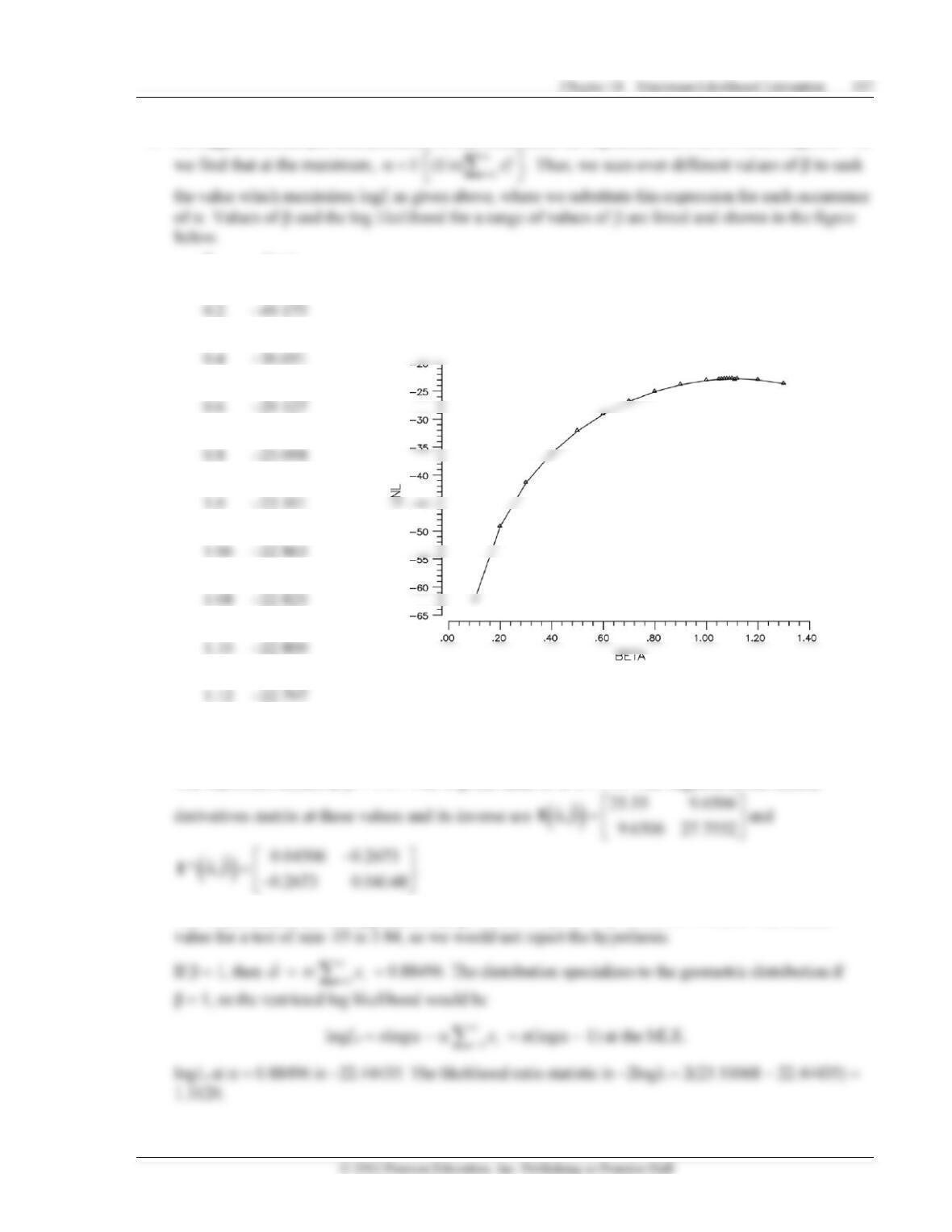
5. As suggested in the previous problem, we can concentrate the log likelihood over . From logL/ = 0,

 logL

0.1 −62.386

0.3 −41.381

0.5 −32.122

0.7 −26.829

0.9 −23.866

1.05 −22.891

1.07 −22.841

1.09 −22.809

1.11 −22.796

1.2 −22.984

1.3 −23.693

The maximum occurs at  = 1.11. The implied value of  is 1.179. The negative of the second

The Wald statistic for the hypothesis that  = 1 is W = (1.11 − 1)2/0.041477 = 0.276. The critical

118 Greene • Econometric Analysis, Seventh Edition

Once again, this is a small value. To obtain the Lagrange multiplier statistic, we would compute

at the restricted estimates of  = 0.88496 and  = 1. Making the substitutions from above, at these

values, we would have

logL/ = 0

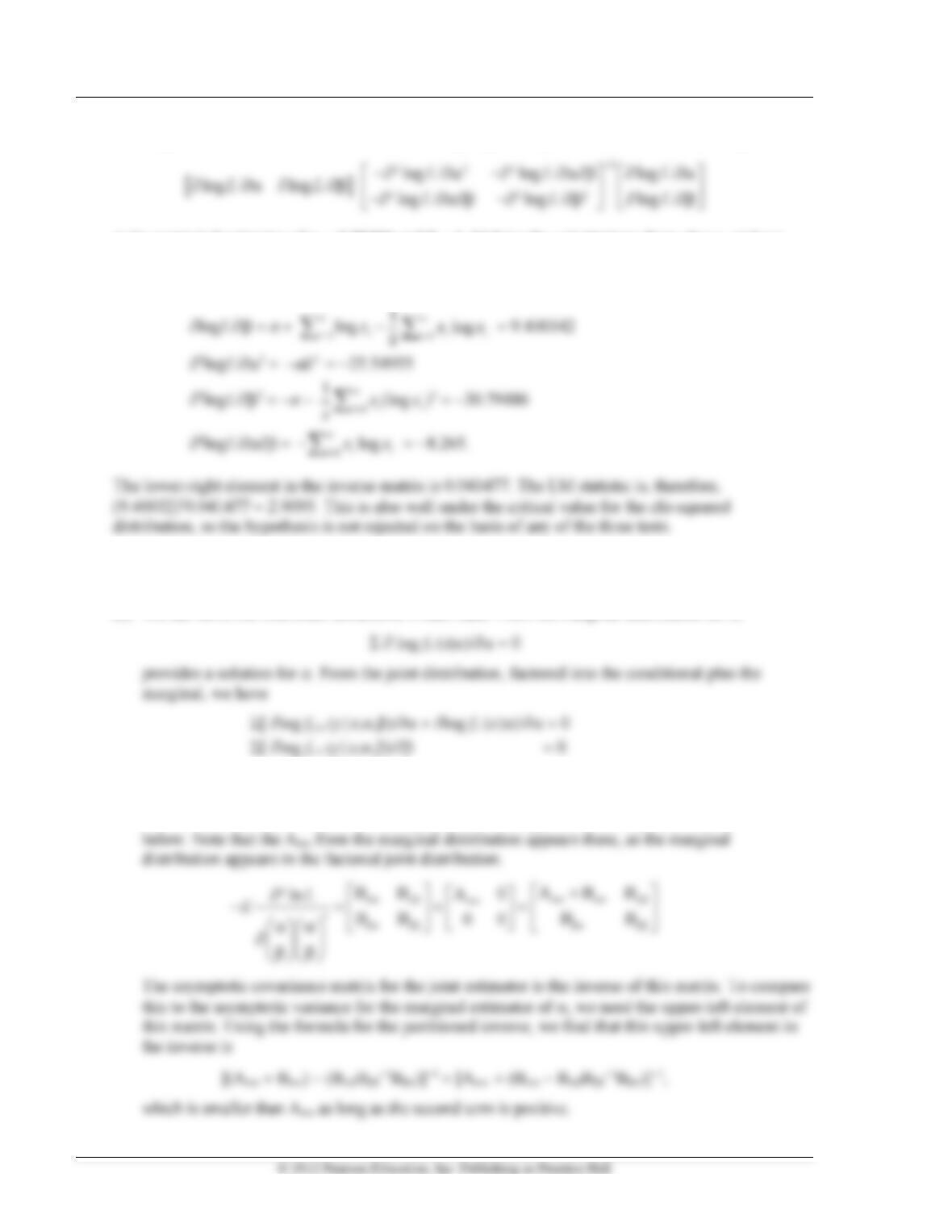
6. (a) The full log likelihood is logL =  log fyx(y,x |,).

(b) By factoring the density, we obtain the equivalent logL = [log fy|x (y|x,,) + log fx (x|)].

(c) We can solve the first-order conditions in each case. From the marginal distribution for x,

(d) The asymptotic variance obtained from the first estimator would be the negative inverse of the

expected second derivative, Asy.Var[a] = {[−E[2 log fx (x |)/2]}−1. Denote this A−1. Now,

consider the second estimator for  and  jointly. The negative of the expected Hessian is shown

Chapter 14 Maximum Likelihood Estimation 119

7. The log likelihood for the Poisson model is

LogL = −n + logi yi − i log yi!.

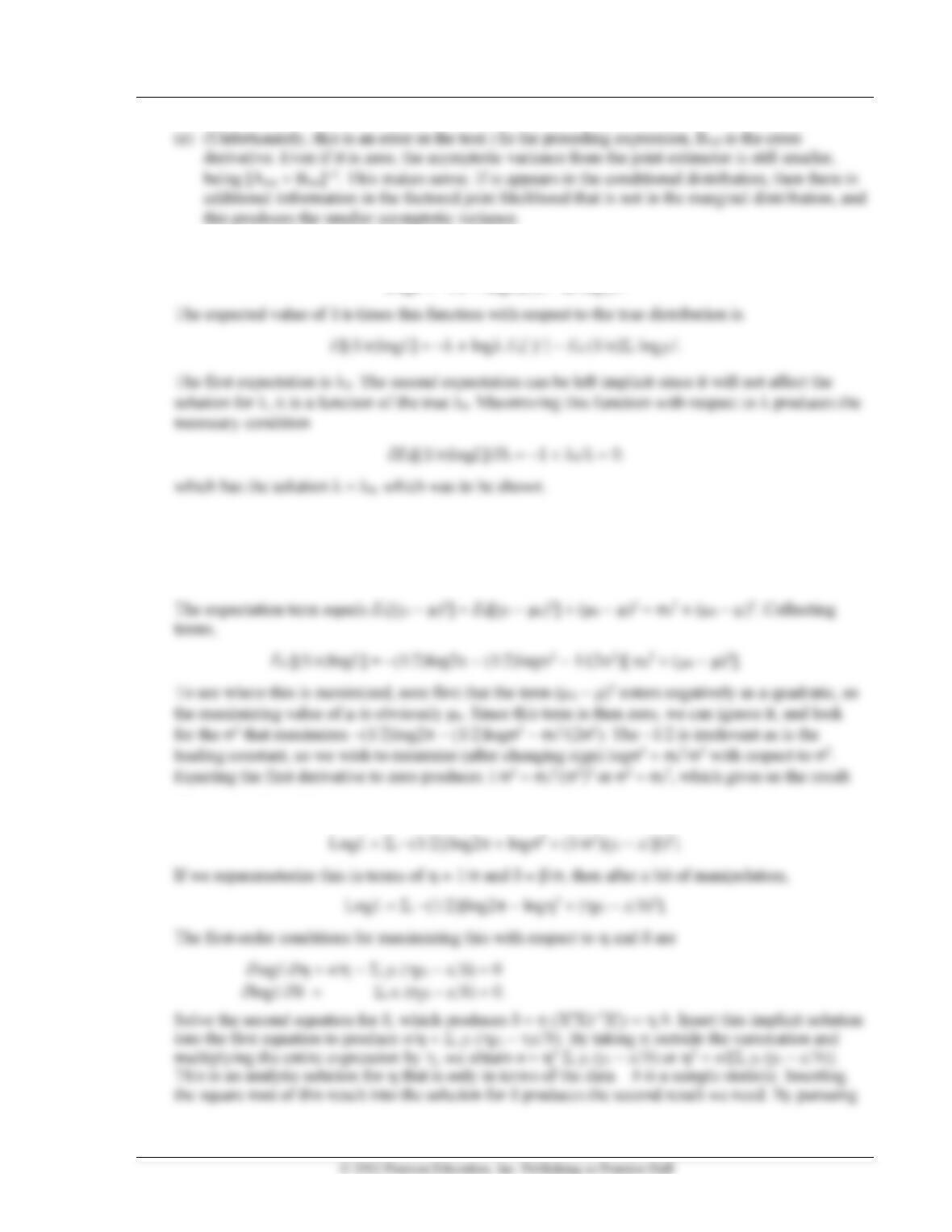
8. The log likelihood for a sample from the normal distribution is

LogL = −(n/2)log2 − (n/2)log2 − 1/(22)i (yi − )2

E0 [(1/n)logL] = −(1/2)log2 − (1/2)log2 − 1/(22) E0[(1/n)i (yi − )2].

9. The log likelihood for the classical normal regression model is

120 Greene • Econometric Analysis, Seventh Edition

this a bit further, you can show that the solution for 2 is just n/ee from the original least squares

regression, and the solution for  is just b times this solution for . The second derivatives matrix is

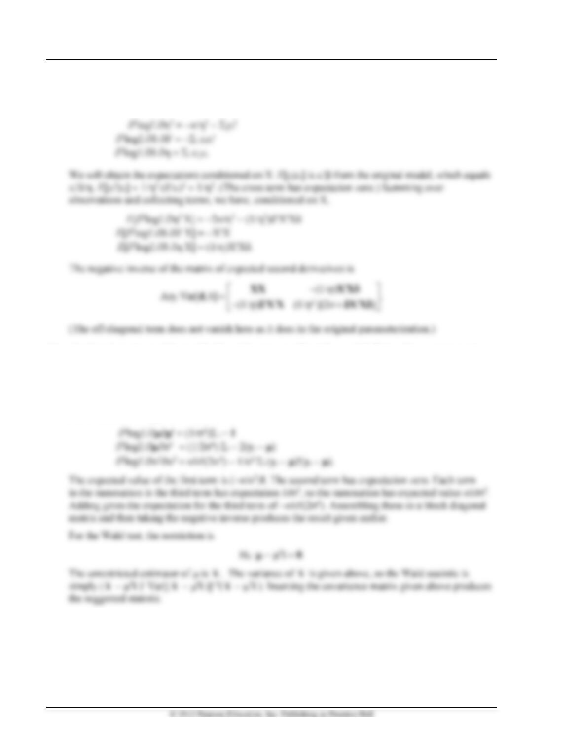
10. The first derivatives of the log likelihood function are logL/ = −(1/22) i − 2(yi − ). Equating

this to zero produces the vector of means for the estimator of . The first derivative with respect

to 2 is logL/2 = −nM/(22) + 1/(24)i (yi − )(yi − ). Each term in the sum is m (yim − m)2.

We already deduced that the estimators of m are the sample means. Inserting these in the solution

for 2 and solving the likelihood equation produces the solution given in the problem. The second

derivatives of the log likelihood are

11. The asymptotic variance of the MLE is, in fact, equal to the Cramér-Rao lower bound for the

variance of a consistent, asymptotically normally distributed estimator, so this completes the

argument.

Chapter 14 Maximum Likelihood Estimation 121

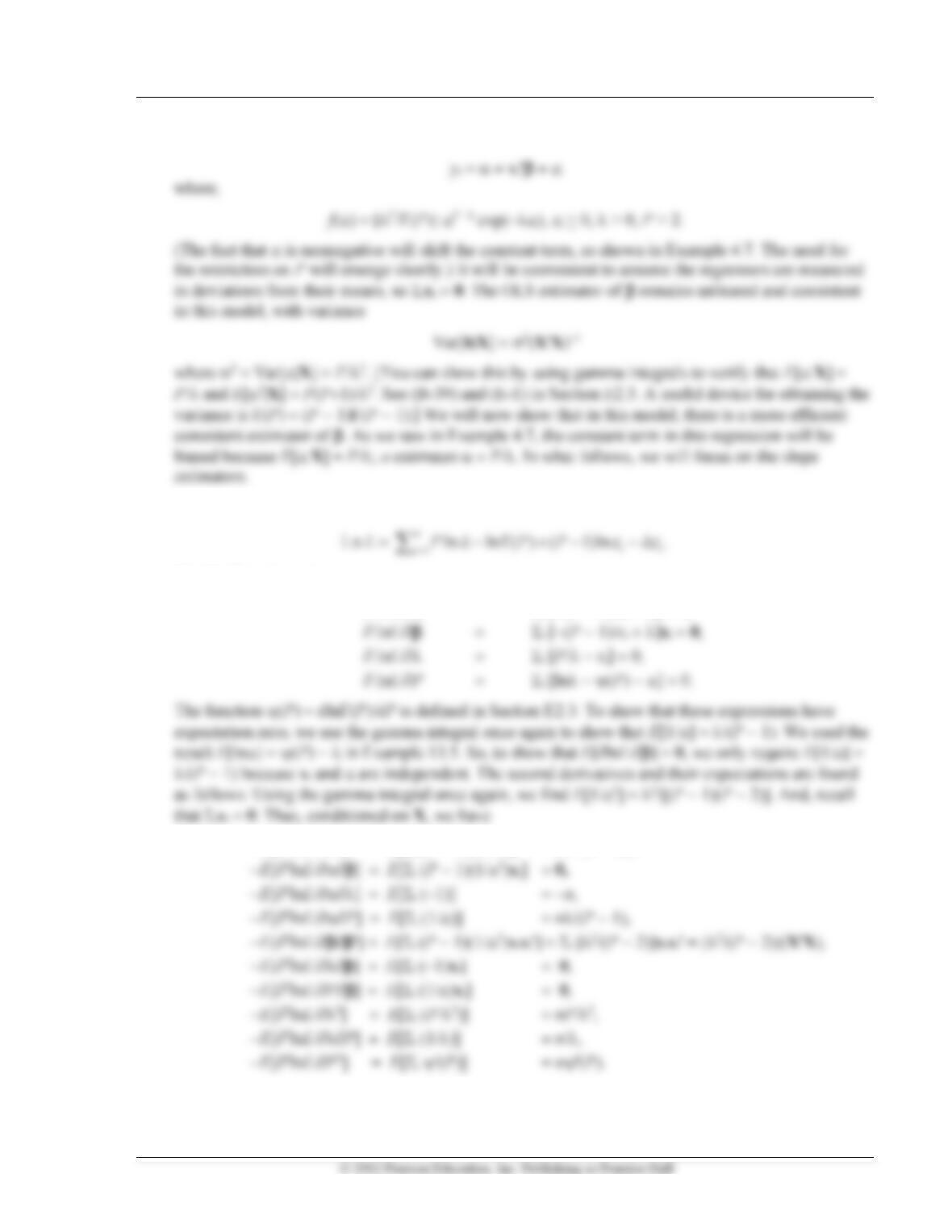
In Example 4.7, we proposed a regression with a gamma distributed disturbance,

The log-likelihood function is

The likelihood equations are

 lnL/ = i [−(P − 1)/



i + ] = 0,

−E[2lnL/2] = E[i (P − 1)(1/



i2)] = n2/(P − 2),

122 Greene • Econometric Analysis, Seventh Edition

Since the expectations of the cross partials with respect to  and the other parameters are all zero, it

follows that the asymptotic covariance matrix for the MLE of  is simply

Applications

1. (a) For both probabilities, the symmetry implies that 1 − F(t) = F(−t). In either model, then,

(b) lnL/ =

=



−−



−

xx

x

1

[(2 1) ] (2 1)

[(2 1) ]

nii

ii

i

ii

fy y

Fy



= 0 where f[(2yi − 1)xi] is the density function.

For the logit model, f = F(1 − F). So, for the logit model,

(c) For the logit model, the result is very simple:

Chapter 14 Maximum Likelihood Estimation 123

(d) Denote by H the actual second derivatives matrix derived in the previous part. Then, Newton’s

method is

(e) The method of scoring uses the expected Hessian instead of the actual Hessian in the iterations.

The methods are the same for the logit model, since the Hessian does not involve yi. The methods

are different for the probit model, since the expected Hessian does not equal the actual one. For

the logit model

124 Greene • Econometric Analysis, Seventh Edition

?====================================================

? Application 14.1(f)

?====================================================

Namelist ; x = one,age,educ,hsat,female,married $

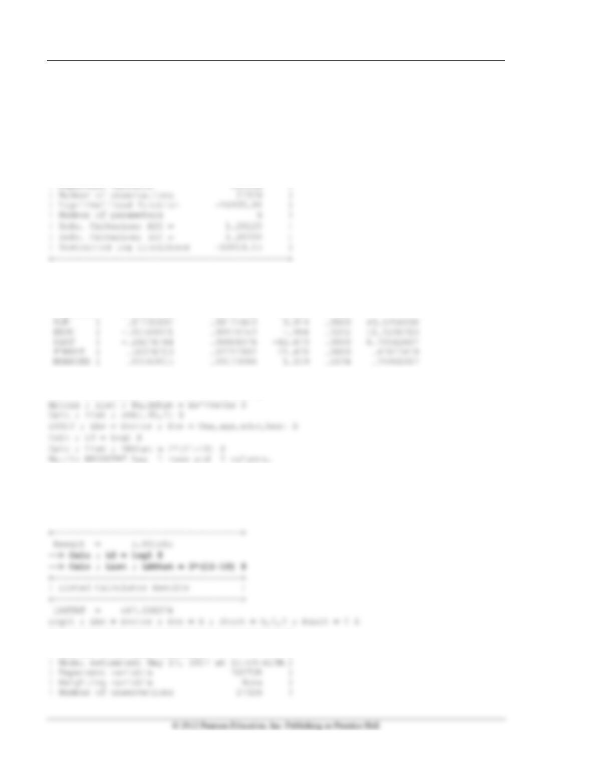
LOGIT ; Lhs = Doctor ; Rhs = X $

Calc ; L1 = logl $

+———————————————+

| Binary Logit Model for Binary Choice |

+——–+————–+—————-+——–+——–+———-+

+——–+————–+—————-+——–+——–+———-+

———+Characteristics in numerator of Prob[Y = 1]

Constant| 1.82207669 .10763712 16.928 .0000

Application 14.1(g)

Matr ; bw = b(5:6) ; vw = varb(5:6,5:6) $

1

+————–

1| 461.43784

–> Calc ; list ; ctb(.95,2) $

+————————————+

| Listed Calculator Results |

+———————————————+

| Binary Logit Model for Binary Choice |

| Maximum Likelihood Estimates |

Chapter 14 Maximum Likelihood Estimation 125

| Iterations completed 1 |

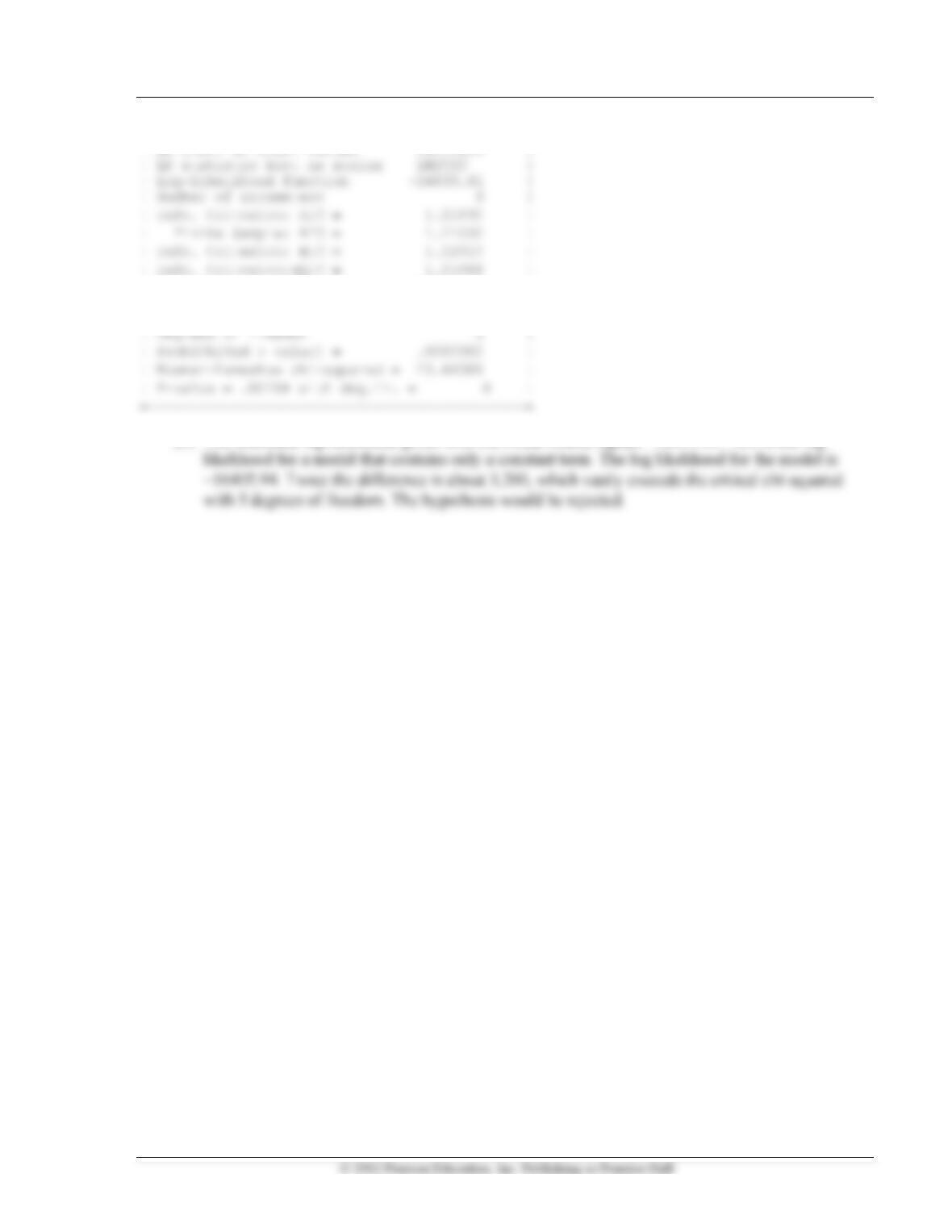
| Restricted log likelihood -18019.55 |

| McFadden Pseudo R-squared .0765802 |

| Chi-squared 2759.883 |

(h) The restricted log likelihood given with the initial results equals −18019.55. This is the log