
Chapter 13 Exchange Rates, Business Cycles, and Macroeconomic Policy in the Open Economy 317
the riskiness of exchange rates changes over time, to make better exchange-rate forecasts. But, so far at
least, short-term exchange rate forecasting is far more an art than a science.
318 Abel/Bernanke/Croushore • Macroeconomics, Ninth Edition
◼ Answers to Textbook Problems
Review Questions
1. The nominal exchange rate is the rate at which two currencies can be exchanged for each other in the
market. The real exchange rate is the price of domestic goods relative to foreign goods. Changes in
2. The two major types of exchange-rate systems are fixed exchange rates and flexible exchange rates.
In a fixed-exchange-rate system, exchange rates are set at officially determined levels. In a flexible-
3. Purchasing power parity, PPP, is the idea that similar foreign and domestic goods, or baskets of
goods, should have the same price when priced in terms of the same currency. Purchasing power
4. The J curve shows the response of net exports to a real depreciation. At first the real depreciation
reduces net exports, as the decline in the real exchange rate means that a country pays more for its
5. An increase in domestic income leads people to buy more goods, including imported goods, so net
exports decline. An increase in foreign income leads foreigners to buy more goods, including goods
6. Foreigners demand dollars in the foreign exchange market to be able to buy U.S. goods and services
(U.S. exports) and U.S. real and financial assets (U.S. capital inflows). Americans supply dollars to
the foreign exchange market to be able to buy foreign goods and services (U.S. imports) and real and
Chapter 13 Exchange Rates, Business Cycles, and Macroeconomic Policy in the Open Economy 319
7. The IS–LM model for the open economy differs from the closed-economy IS–LM model in that
international influences may shift the IS curve. Factors that raise a country’s net exports, given
8. Expansionary fiscal policy increases output and the real interest rate in the short run (using a
Keynesian model), both of which lead to a reduction of net exports. Expansionary monetary policy
9. In the short run, expansionary monetary policy increases output (using a Keynesian model), which
decreases net exports, leading to an increased supply of the domestic currency in the foreign
exchange market, causing it to depreciate. Expansionary monetary policy also reduces the real
10. The fundamental value of a currency is the value of the exchange rate that would be determined by
free-market forces of demand and supply without government intervention. When the official
11. A country is limited in changing its money supply under a fixed-exchange-rate system, because
only one level of the money supply is consistent with the official exchange rate being equal to its
12. Flexible exchange rates have the advantage of allowing a country to use expansionary monetary
policy to combat recessions, but currency values fluctuate substantially, introducing uncertainty
into international transactions. Fixed exchange rates avoid this problem, but a country may have to
320 Abel/Bernanke/Croushore • Macroeconomics, Ninth Edition
Numerical Problems
1. The price level in the West is PW = 5 guilders per ordinary soap bar. The price level in the East is
PE = 100 florins per deluxe soap bar. The real exchange rate is 2 ordinary soap bars per deluxe
soap bar.
2. (a) Japan imports 64 barrels of oil, worth 16 cameras at 4 barrels of oil per camera. It exports
40 cameras, so the real value of its net exports is 24 cameras.
3. Begin by writing the equation for the IS curve, which is Sd − Id = NX.
Sd = Y − Cd − G = Y − (300 + 0.5Y − 200r) − G.
NX = 150 − 0.1Y − 0.5e = 150 − 0.1Y − 0.5(20 + 600r) = 140 − 0.1Y − 300r.
Using these in the IS curve equation gives:
4. (a) Begin by writing the equation for the IS curve, which is Sd − Id = NX.
NX = 150 − 0.08Y − 500r.
Sd = Y − Cd − G = Y − {200 + 0.6[Y − (20 + 0.2Y)] − 200r} − G = 0.52Y − (188 + G) + 200r.
Chapter 13 Exchange Rates, Business Cycles, and Macroeconomic Policy in the Open Economy 321
0.6(1000 − 220) − 38 = 630, and I = 300 − 57 = 243.
(b) In the short run with G = 214 and P = 2, the IS curve now gives 1000r = (638 + 214) − 0.6Y, and
the LM curve is 200r = 0.5Y − 462. Take five times the LM equation and subtract it from the IS
10.4, while G is 62 lower, or 152. In the long run, NX is 62 higher than before (NX = 6), while
G is 62 lower at 152.
5. (a) AD intersects AS at 1000 = 400 + 50M/P, which means M/P = 12. With M = 48 francs, P = 4
6. (a) c0 = 200, cY = 0.6, t0 = 20, t
=
0.2, cr = 200
i0 = 300, ir= 300
x0 =150, xY = 0.08, xYF = 0, xr = 500, xrF = 0
322 Abel/Bernanke/Croushore • Macroeconomics, Ninth Edition
LM = 0.5/200 = 0.0025
(c) In general equilibrium, Y = 1000, so
IS: r = 0.79 − (0.0006 1000) = 0.19
LM: r = 0 − (1/200)924/P + (0.0025 1000), so 4.62/P = 2.31, so P = 2.
Chapter 13 Exchange Rates, Business Cycles, and Macroeconomic Policy in the Open Economy 323
Analytical Problems
1. (a) The temporary import restriction increases net exports. Since it raises the demand for domestic
goods relative to foreign goods, the real exchange rate increases. The rise in the exchange rate
mitigates somewhat the increase in net exports caused by the restriction, but the latter
dominates, so net exports rise.
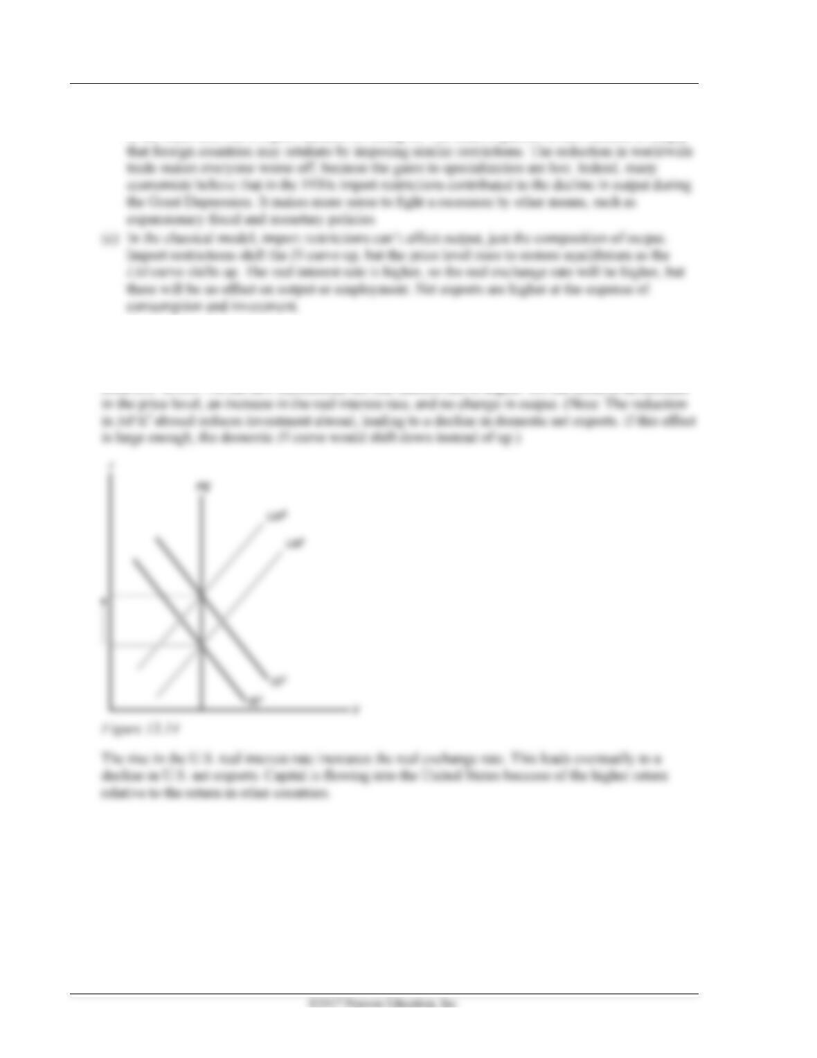
Suppose the economy is initially in a recession at the intersection of the IS1 and LM curves in
(b) Since the restriction increases the home country’s net exports, it must decrease foreign
countries’ net exports. This is shown by the shift to the left of the IS curve from IS1 to IS2 in
Figure 13.13. Thus output and the real interest rate decline in the foreign country. The fall in
output leads to a decline in employment. The price level is unchanged in the short run. The
foreign currency depreciates, since the domestic currency appreciates.
324 Abel/Bernanke/Croushore • Macroeconomics, Ninth Edition
Although the results of this exercise indicate that import restrictions can be used to fight recessions
in the short run, this is a poor method for doing so. The main objection to this method is simply
2. The fall in the MPKf abroad and the rise in the MPKf in the United States increases U.S. investment
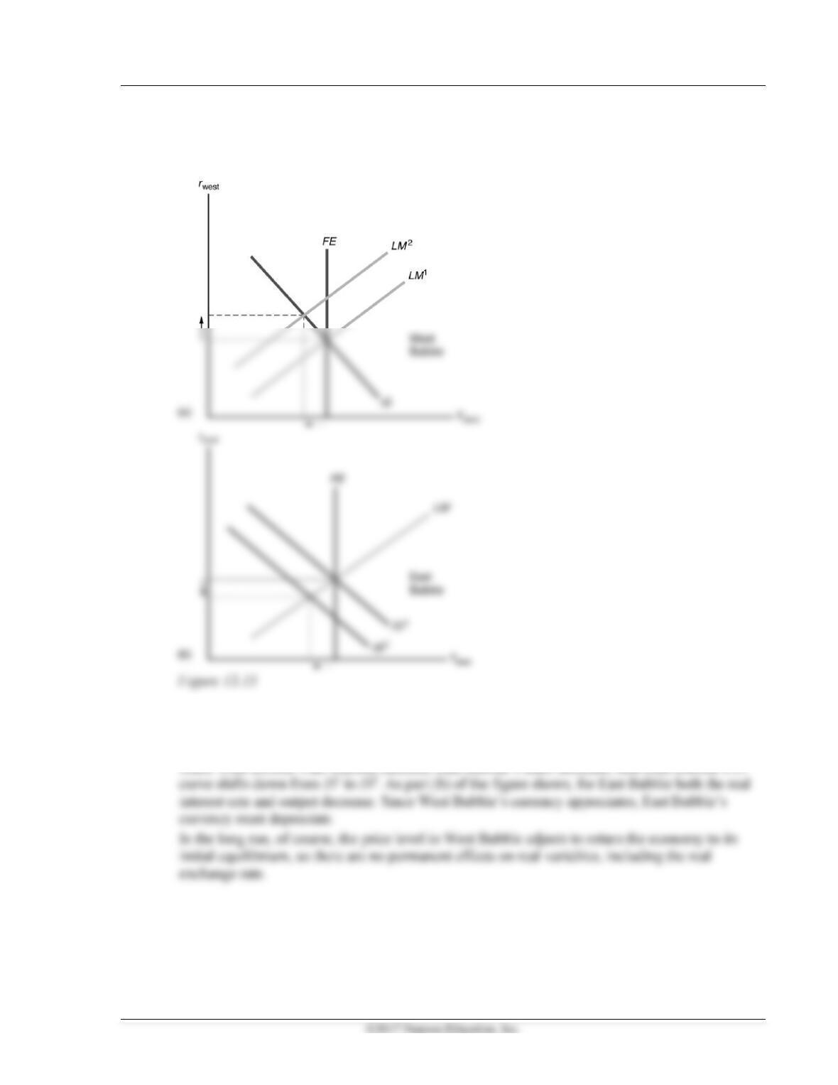
for any given real interest rate, shifting the IS curve up and to the right. This is shown in Figure
13.14 as a shift from IS1 to IS2. To restore equilibrium, prices must rise so that the LM curve shifts up
from LM1 to LM2. At the new equilibrium the real interest rate is higher. So, the result is an increase
Chapter 13 Exchange Rates, Business Cycles, and Macroeconomic Policy in the Open Economy 325
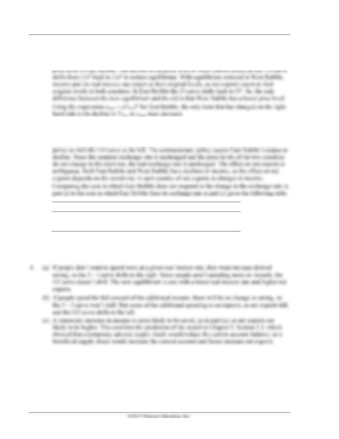
3. (a) West Bubble’s contractionary monetary policy shifts its LM curve up and to the left, from LM1
to LM2 in part (a) of Figure 13.15. The intersection of the IS and LM curves is one in which
output is below full-employment output and the real interest rate is higher than before.
The decrease in West Bubble’s output increases its net exports. The higher real interest rate
causes the currency to appreciate, which decreases its net exports. It is likely that the reduction
in income increases net exports by more. So, West Bubble’s net exports rise.
Since West Bubble’s net exports increase, East Bubble’s must decrease, thus East Bubble’s IS
326 Abel/Bernanke/Croushore • Macroeconomics, Ninth Edition
(b) In the short run East Bubble’s real exchange rate decreases, and since the price level does not
change in the short run, East Bubble’s nominal exchange rate must also decrease [since enom =
ePFor/P]. In the long run the price level declines in West Bubble, but there is no effect on the
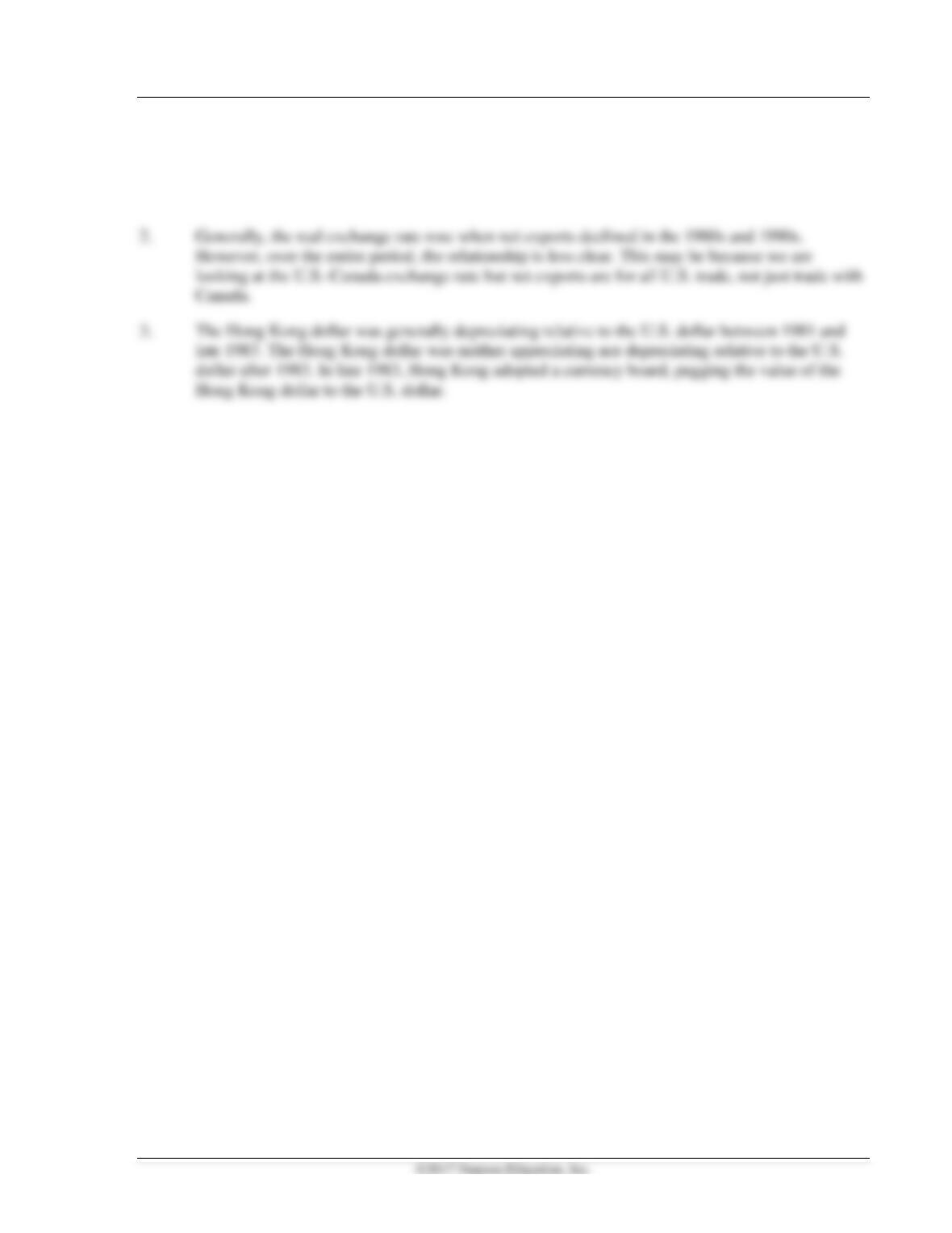
(c) If East Bubble wants to offset West Bubble’s contractionary policy to keep it from affecting the
exchange rate, it must also use contractionary policy. When West Bubble uses contractionary
policy, East Bubble’s IS curve shifts down, because its net exports decline. To prevent the
nominal exchange rate from declining, East Bubble must itself use contractionary monetary
Output
Real Exchange Rate
Net Exports
No response
falls
falls
fall
Fix exchange rate
falls
no change
uncertain
(d) If East Bubble doesn’t change its macroeconomic policies, its currency will become overvalued.
Then it must devalue the currency, impose restrictions on international transactions, or support
the currency by buying it in the foreign exchange market, losing official reserve assets.
Chapter 13 Exchange Rates, Business Cycles, and Macroeconomic Policy in the Open Economy 327
Working with Macroeconomic Data
1. a. Real exchange-rate fluctuations arise primarily from nominal exchange-rate fluctuations.
b. In the data, the relationship between the real interest rate and the exchange rate is not clear.
328 Abel/Bernanke/Croushore • Macroeconomics, Ninth Edition
◼ The IEB-IRP Model
The real exchange rate, the quantity of foreign goods that can be acquired in exchange for one unit of
the domestic good, is an important determinant of a country’s net exports and therefore of domestic
The International Flow of Goods: Intertemporal External Balance
As discussed in Chapter 5, a country with positive net exports produces more goods than are purchased
by its consumers, firms, and governments. The country’s excess of output over spending equals its
lending to other countries. In the future the country will be paid back what it has lent with interest, which
will allow it to spend more than it produces and have negative net exports.
The requirement that countries that have positive net exports and lend today have negative net exports
in the future—and similarly, that countries that have negative net exports and borrow today have positive
net exports in the future—is known as intertemporal external balance. (External refers to the flows
of goods across international borders, and intertemporal emphasizes that the flow of goods between
countries need not balance in every period but must balance over time.) Put simply, intertemporal
In general, for a country to achieve external balance, its future net exports NXf must equal −(1 + r)NX,
where NX is current net exports and r is the real interest rate. (For simplicity, we continue to assume two
periods.) In our example NX = −100 and r = 0.08, so NXf = 108, as we found. Alternatively, suppose that
the country’s current net exports were positive and equal to 100 home goods. With net exports of 100
that period, as well as on other factors. [Those readers who covered Chapter 8 will recognize that