156
CHAPTER 13
TEACHING NOTES
While this chapter falls under “Advanced Topics,” most of this chapter requires no more
sophistication than the previous chapters. (In fact, I would argue that, with the possible
exception of Section 13.5, this material is easier than some of the time series chapters.)
Two years of panel data are often available, in which case differencing across time is a simple
way of removing g unobserved heterogeneity. If you have covered Chapter 9, you might
compare this with a regression in levels using the second year of data, but where a lagged
dependent variable is included. (The second approach only requires collecting information on
the dependent variable in a previous year.) These often give similar answers. Two years of
panel data, collected before and after a policy change, can be very powerful for policy analysis.

157
SOLUTIONS TO PROBLEMS
13.1 Without changes in the averages of any explanatory variables, the average fertility rate fell
by .545 between 1972 and 1984; this is simply the coefficient on y84. To account for the
13.2 The first equation omits the 1981 year dummy variable, y81, and so does not allow any
appreciation in nominal housing prices over the three year period in the absence of an
incinerator. The interaction term in this case is simply picking up the fact that even homes that
13.3 We do not have repeated observations on the same cross-sectional units in each time period,
and so it makes no sense to look for pairs to difference. For example, in Example 13.1, it is very
13.4 The sign of 1 does not affect the direction of bias in the OLS estimator of
1
, but only
13.5 No, we cannot include age as an explanatory variable in the original model. Each person in
the panel data set is exactly two years older on January 31, 1992 than on January 31, 1990. This
158
13.6 (i) Let FL be a binary variable equal to one if a person lives in Florida, and zero otherwise.
Let y90 be a year dummy variable for 1990. Then, from equation (13.10), we have the linear
probability model
(ii) It could be that the populations of drivers in the two states change in different ways over
time. For example, age, race, or gender distributions may have changed. The levels of education
13.7 (i) It is not surprising that the coefficient on the interaction term changes little when
afchnge is dropped from the equation because the coefficient on afchnge in (3.12) is only .0077
(and its t statistic is very small). The increase from .191 to .198 is easily explained by sampling
error.
(ii) If highearn is dropped from the equation [so that
10
=
in (3.10)], then we are assuming
SOLUTIONS TO COMPUTER EXERCISES
C13.1 (i) The F statistic (with 4 and 1,111 df) is about 1.16 and p-value
.328, which shows
that the living environment variables are jointly insignificant.
159
df, the p-value is about .0082. So there is evidence of heteroskedasticity that is a function of
(iv) Adding y74
educ, , y84
educ allows the relationship between fertility and education
to be different in each year; remember, the coefficient on the interaction gets added to the
coefficient on educ to get the slope for the appropriate year. When these interaction terms are
added to the equation, R2
.137. The F statistic for joint significance (with 6 and 1,105 df) is
C13.2 (i) The coefficient on y85 is roughly the proportionate change in wage for a male
(female = 0) with zero years of education (educ = 0). This is not especially useful because the
U.S. working population without any education is a small group; such people are in no way
“typical.”
(ii) What we want to estimate is
0 =
0 + 12
1; this is the change in the intercept for a male
160
(7.10), which implies the point estimate 40.4%; but obtaining the standard error of this estimate
is harder.)
(iii) Only the coefficient on y85 differs from equation (13.2). The new coefficient is about
(iv) The R-squared when log(rwage) is the dependent variable is .356, as compared with .426
(v) In 1978, about 30.6% of workers in the sample belonged to a union. In 1985, only about
18% belonged to a union. Therefore, over the seven-year period, there was a notable fall in
union membership.
(vi) When y85
union is added to the equation, its coefficient and standard error are about
C13.3 (i) Other things equal, homes farther from the incinerator should be worth more, so 1 > 0.
If 1 > 0, then the incinerator was located farther away from more expensive homes.
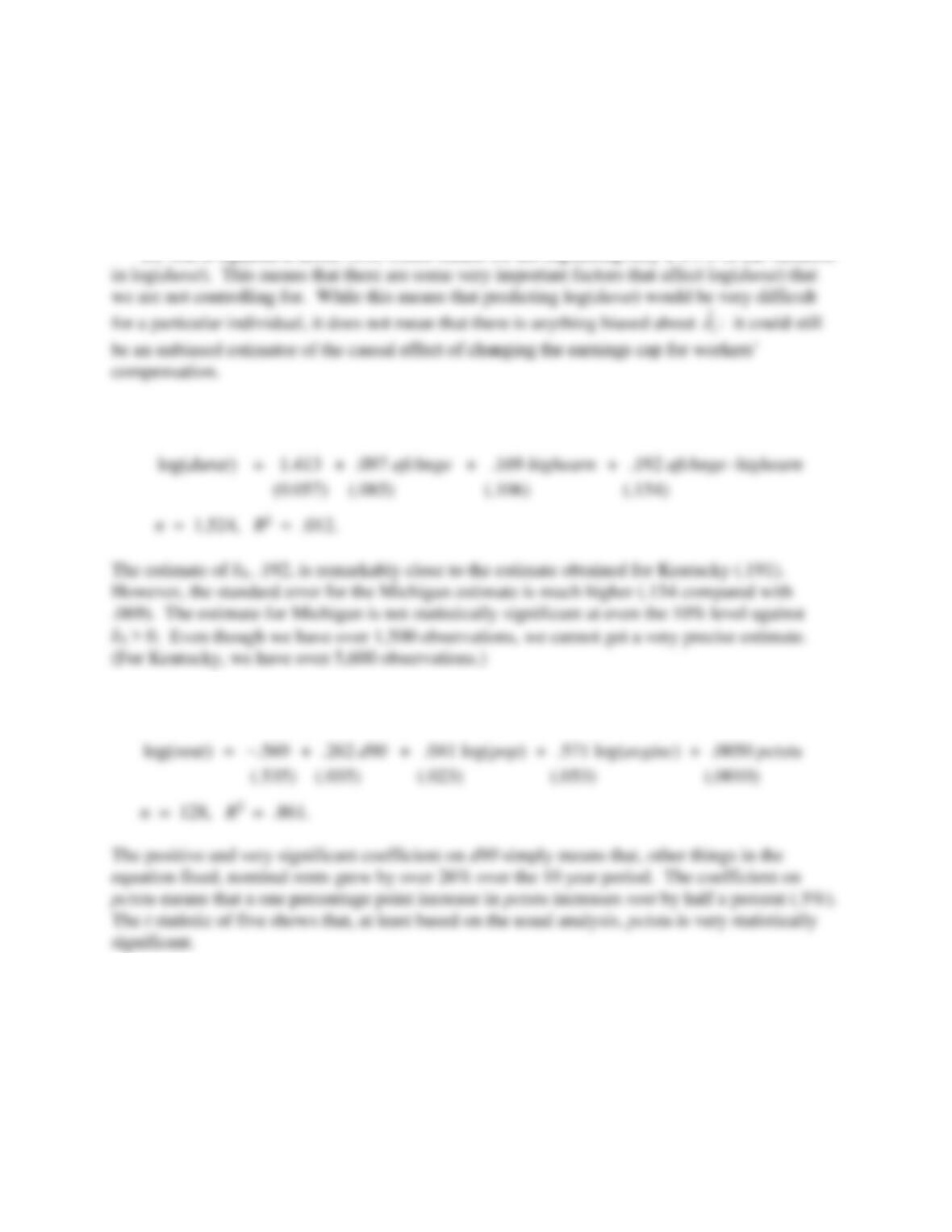
(ii) The estimated equation is
161
C13.4 (i) In addition to male and married, we add the variables head, neck, upextr, trunk,
lowback, lowextr, and occdis for injury type, and manuf and construc for industry. The
coefficient on afchnge
highearn becomes .231 (se
.070), and so the estimated effect and t
statistic are now larger than when we omitted the control variables. The estimate .231 implies a
substantial response of durat to the change in the cap for high-earnings workers.
(ii) The R-squared is about .041, which means we are explaining only a 4.1% of the variation
(iii) The estimated equation using the Michigan data is
C13.5 (i) Using pooled OLS we obtain
(ii) The standard errors from part (i) are not valid, unless we thing ai does not really appear in
the equation. If ai is in the error term, the errors across the two time periods for each city are
positively correlated, and this invalidates the usual OLS standard errors and t statistics.
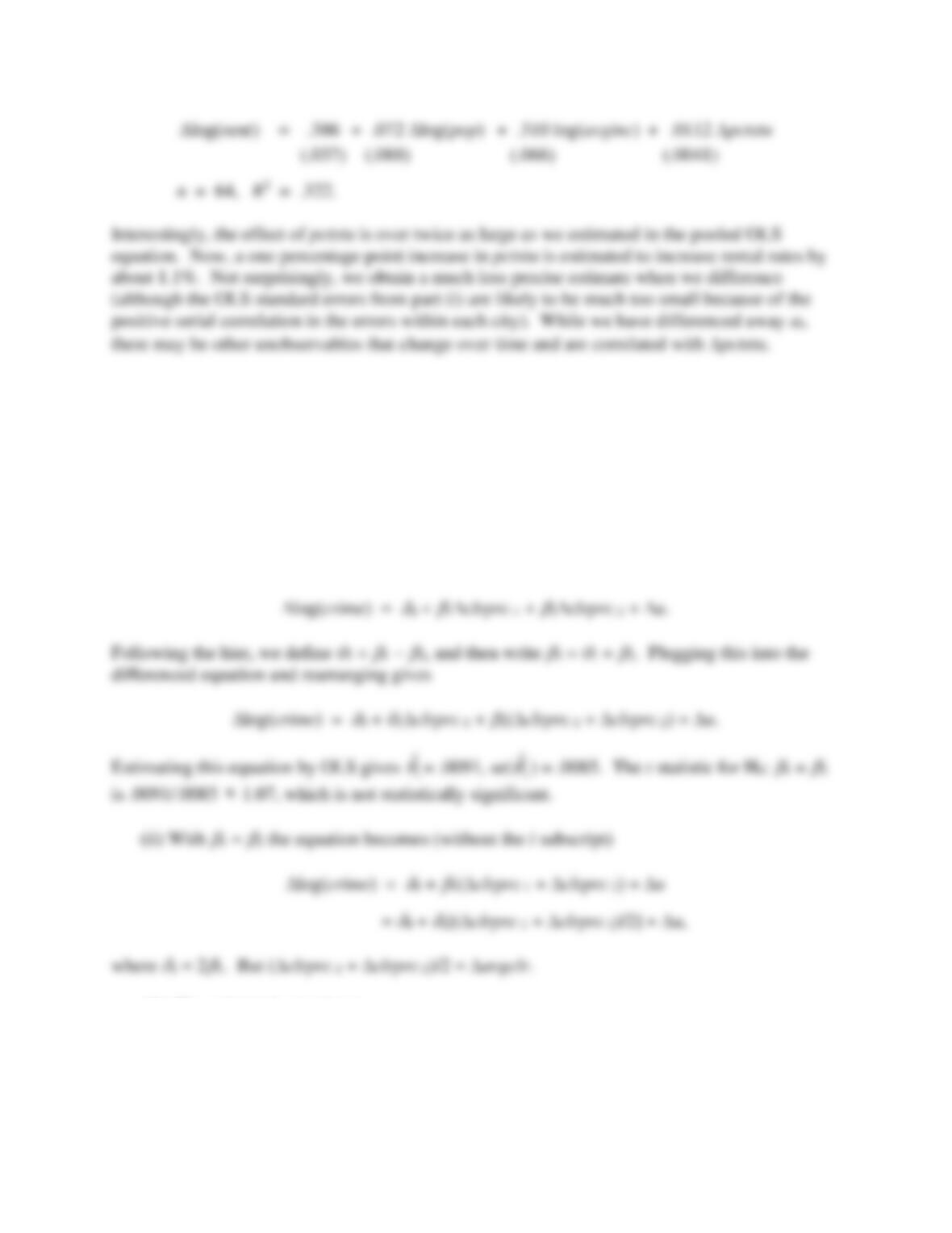
(iii) The equation estimated in differences is
162
(iv) The heteroskedasticity-robust standard error on pctstu is about .0028, which is actually
much smaller than the usual OLS standard error. This only makes pctstu even more significant
(robust t statistic
4). Note that serial correlation is no longer an issue because we have no time
component in the first-differenced equation.
C13.6 (i) You may use an econometrics software package that directly tests restrictions such as
H0:
1 =
2 after estimating the unrestricted model in (13.22). But, as we have seen many times,
we can simply rewrite the equation to test this using any regression software. Write the
differenced equation as
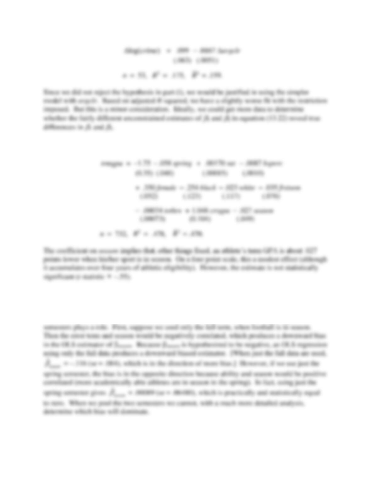
(iii) The estimated equation is
163
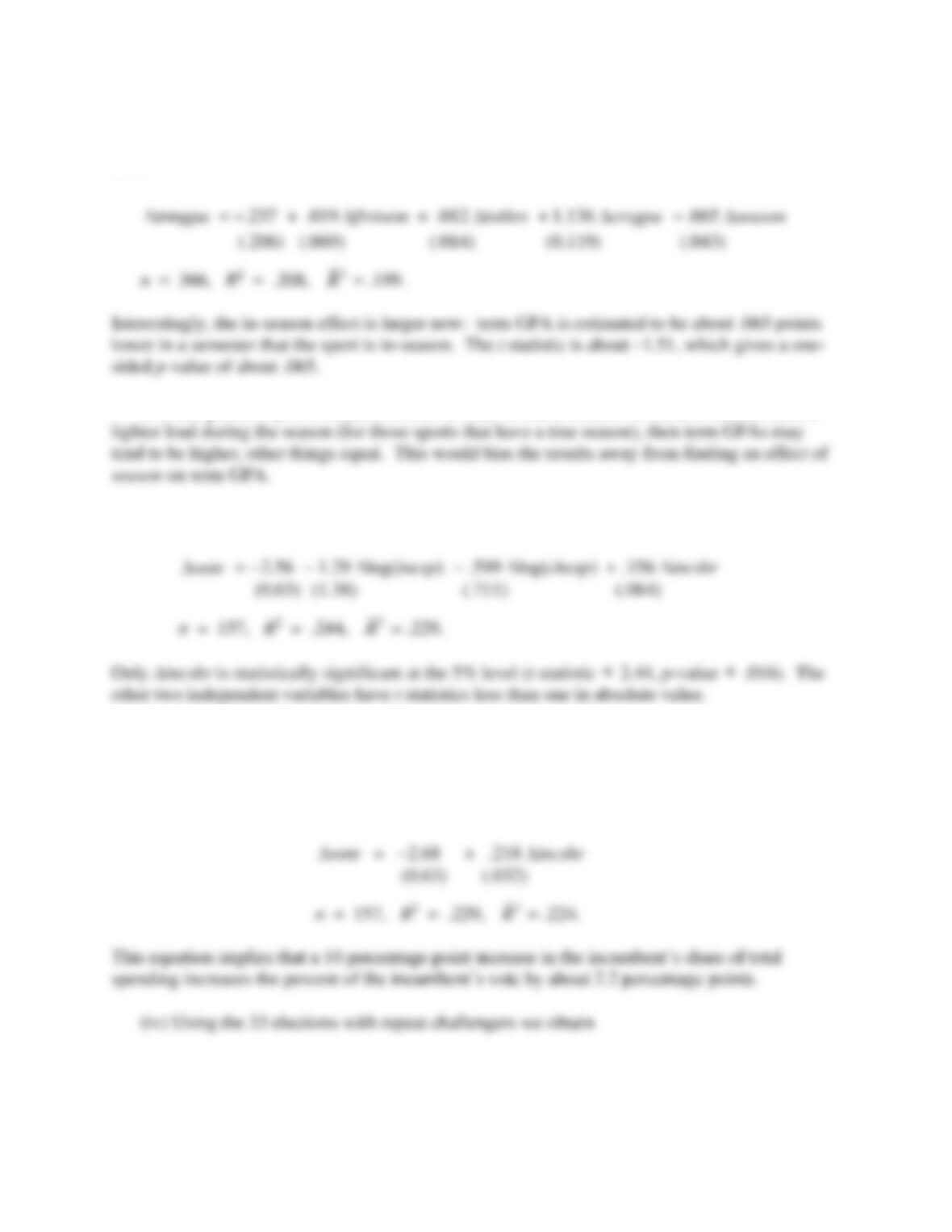
C13.7 (i) Pooling across semesters and using OLS gives
(ii) The quick answer is that if omitted ability is correlated with season then, as we know
from Chapters 3 and 5, OLS is biased and inconsistent. The fact that we are pooling across two
semesters does not change that basic point.
If we think harder, the direction of the bias is not clear, and this is where pooling across
164
(iii) The variables sat, hsperc, female, black, and white all drop out because they do not vary
by semester. The intercept in the first-differenced equation is the intercept for the spring. We
have
(iv) One possibility is a measure of course load. If some fraction of student-athletes take a
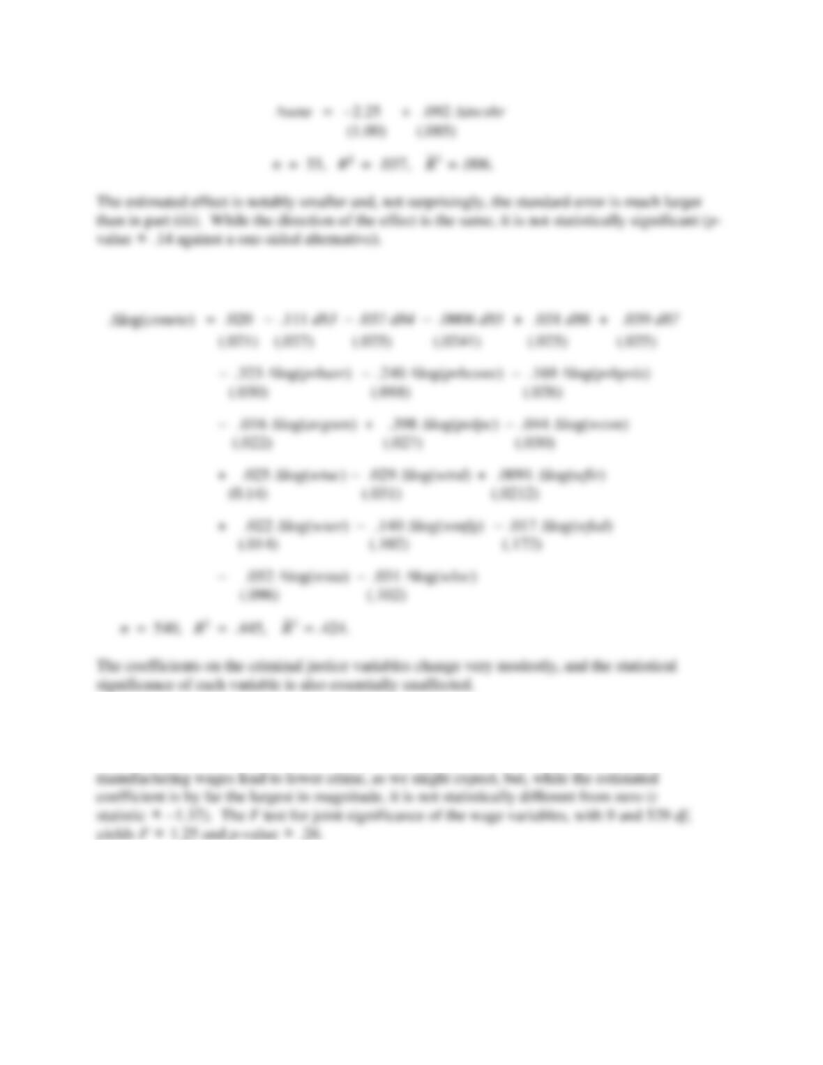
C13.8 (i) The estimated equation using differences is
(ii) The F statistic (with 2 and 153 df) is about 1.51 with p-value
.224. Therefore,
log(inexp) and log(chexp) are jointly insignificant at even the 20% level.
(iii) The simple regression equation is
165
C13.9 (i) When we add the changes of the nine log wage variables to equation (13.33) we obtain
(ii) Since some signs are positive and others are negative, they cannot all really have the
expected sign. For example, why is the coefficient on the wage for transportation, utilities, and
communications (wtuc) positive and marginally significant (t statistic
1.79)? Higher
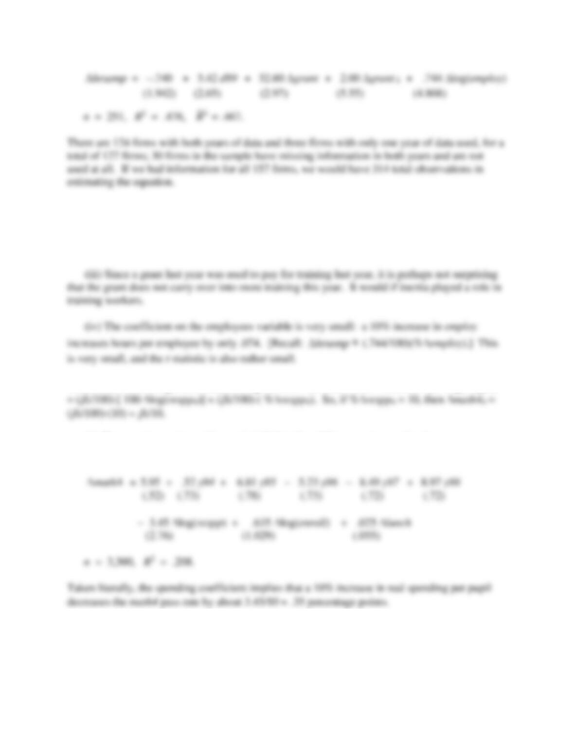
C13.10 (i) The estimated equation using the 1987 to 1988 and 1988 to 1989 changes, where we
include a year dummy for 1989 in addition to an overall intercept, is
166
(ii) The coefficient on grant – more precisely, on grant in the differenced equation – means
that if a firm received a grant for the current year, it trained each worker an average of 32.6 hours
more than it would have otherwise. This is a practically large effect, and the t statistic is very
large.
C13.11. (i) Take changes as usual, holding the other variables fixed: math4it =
1log(rexppit)
(ii) The equation, estimated by pooled OLS in first differences (except for the year
dummies), is
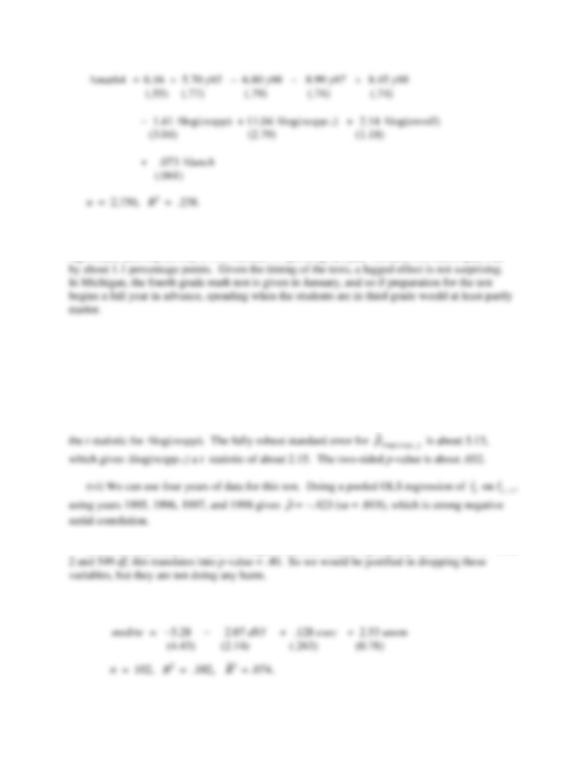
(iii) When we add the lagged spending change, and drop another year, we get
167
The contemporaneous spending variable, while still having a negative coefficient, is not at all
statistically significant. The coefficient on the lagged spending variable is very statistically
significant, and implies that a 10% increase in spending last year increases the math4 pass rate
(iv) The heteroskedasticity-robust standard error for
log( )
ˆrexpp
is about 4.28, which reduces
the significance of log(rexpp) even further. The heteroskedasticity-robust standard error of
1
log( )
ˆrexpp
−
is about 4.38, which substantially lowers the t statistic. Still, log(rexpp-1) is
statistically significant at just over the 1% significance level against a two-sided alternative.
(v) The fully robust standard error for
log( )
ˆrexpp
1
log( )
ˆrexpp
−
is about 4.94, which even further reduces
(vii) The fully robust “F” test for log(enroll) and lunch, reported by Stata 7.0, is .93. With
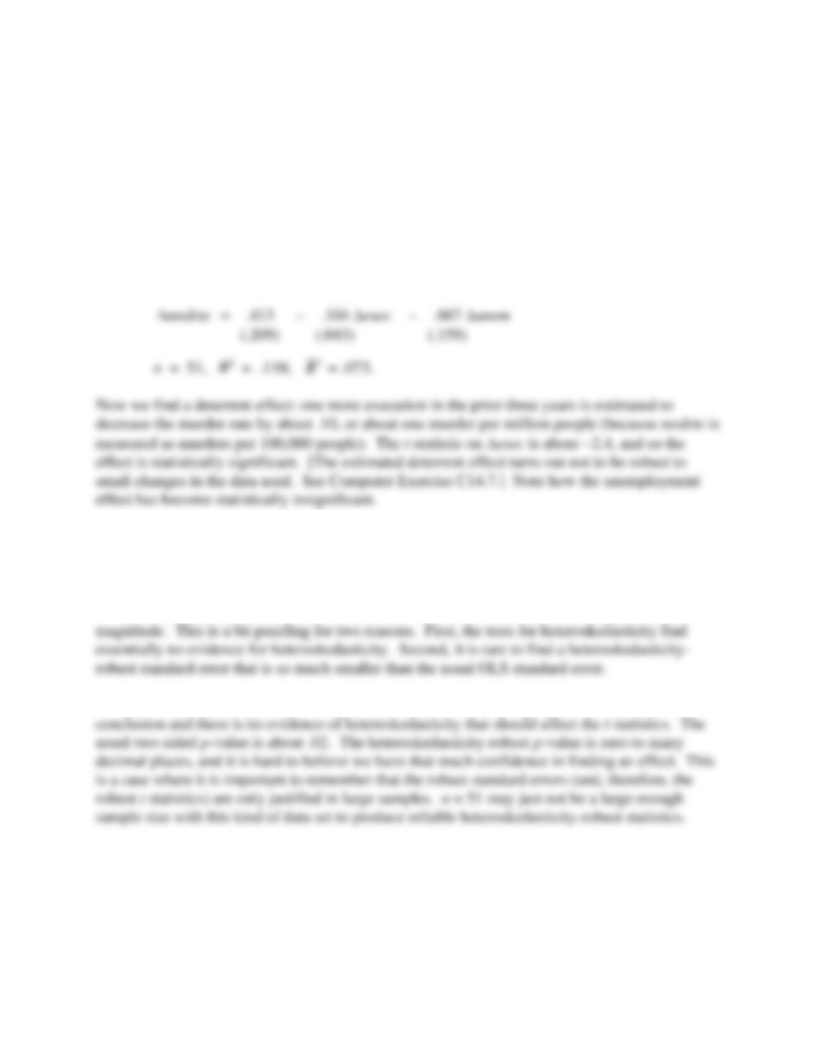
C13.12. (i) The estimated equation using pooled OLS is
168
Because the coefficient on exec is positive (but statistically insignificant), there is no evidence of
a deterrent effect. In using pooled OLS, we are exploiting only the cross-sectional variation in
the data. If states that have had high murder rates in the past have reacted by implementing
capital punishment, we can see a positive relationship between murder rates and capital
punishment even if there is a deterrent effect. (Yet again, we must distinguish between
correlation and causality.)
(ii) If we difference away the unobserved state effects – which can include historical factors
that lead to higher murder rates and aggressive use of capital punishment – the story is different.
The FD estimates are
(iii) The BP and White tests both test two restrictions in this case. The BP F statistic is .60
and the White F statistic is .58. Both have p-values above .50, so there is no evidence of
heteroskedasticity in the FD equation.
(iv) The heteroskedasticity-robust t statistic on exec is −6.11, which is a huge increase in
(v) I would tend to go with the usual OLS t statistic because it gives a more cautious
C13.13 (i) We can estimate all parameters except
0
and
1
: the intercept for the base year
cannot be estimated, and neither can coefficients on the time-constant variable educi.
169
(ii) We want to test
0 1 2 7
: ,..., 0H
==
, so there are seven restrictions to be tested. Using
(iv) The estimated union differential in 1980 is simply the coefficient on
it
union
, or about
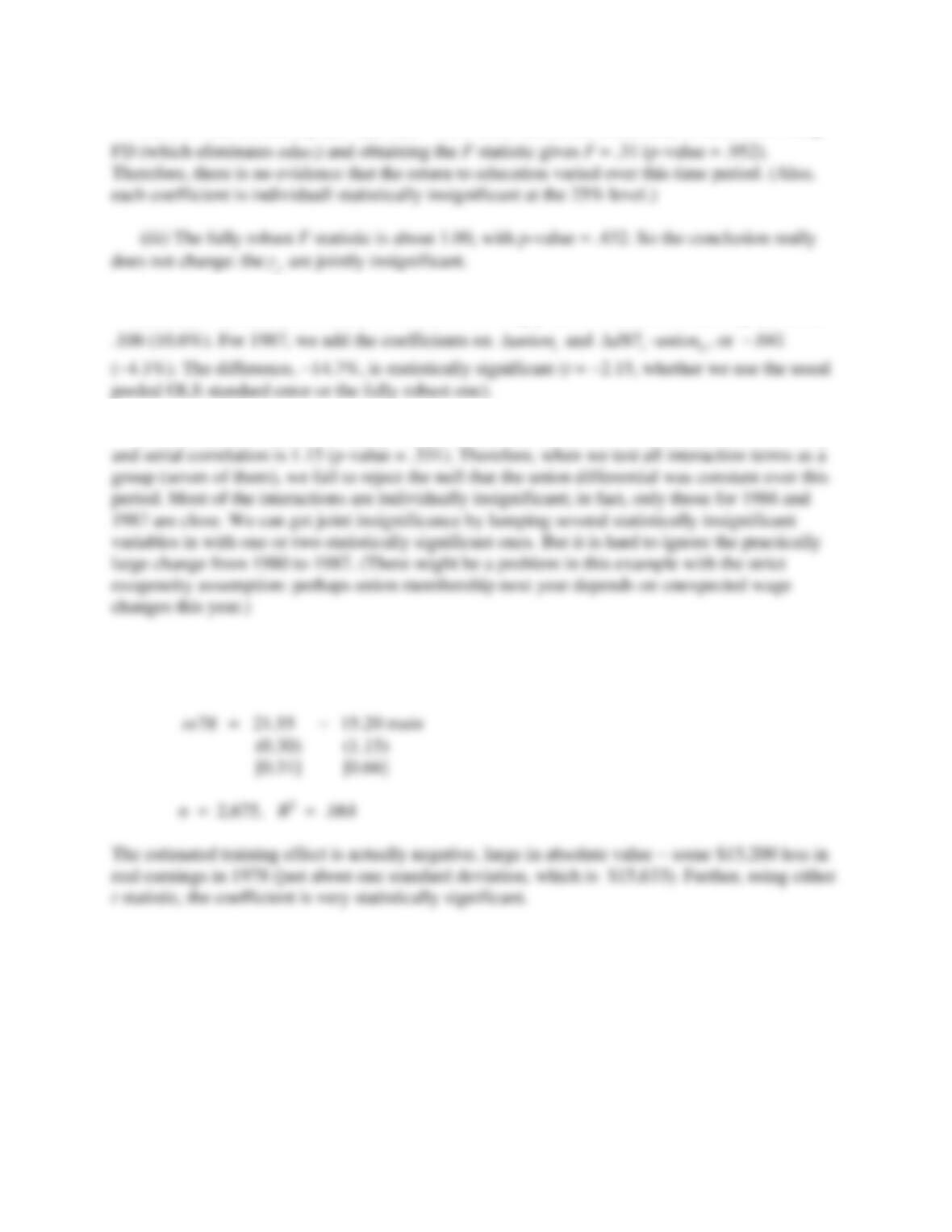
(v) The usual F statistic is 1.03 (p-value = .405) and the statistic robust to heteroskedasticity
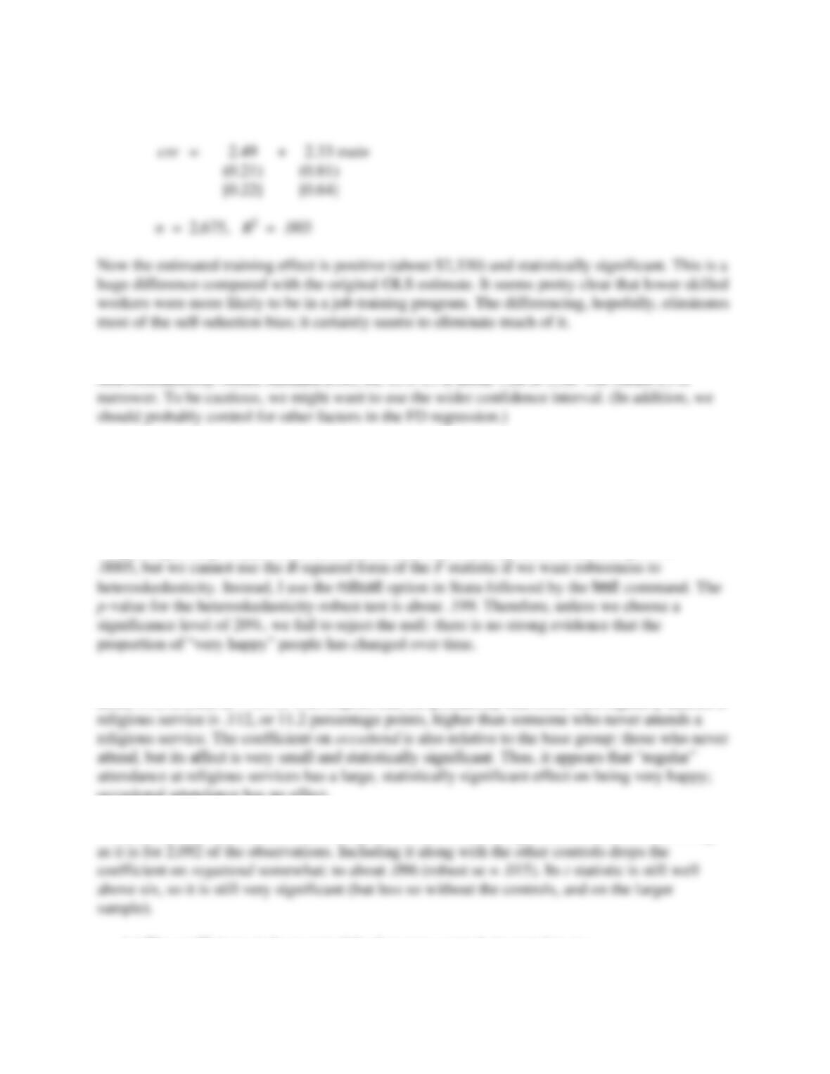
C13.14 (i) The simple regression estimates, with usual OLS standard errors in () and
heteroskedasticity-robust standard errors in [], are
170
(ii) With cre = re78 − re75, the simple regression results are
(iii) The 95% CI using the usual OLS standard error is about .74 to 3.92. Using the
C13.15 (i) Tabulation the observations by year, the year with the most number of observations is
the most recent, 2006 (2,986 people). The year with the fewest observation is 2004 with only
1,337 people. Out of 17,137 total people in the sample, 5,260, or about 30.69%, report being
“very happy.”
(ii) Regressing vhappy on the year dummies y96, y98, y00, y02, y04, and y06 gives R2 =
(iii) The coefficient on occattend is about .0043 (robust se = .0080) and that on regattend is
about .112 (robust se = .011). This implies that the probability that some who regularly attends a
occasional attendance has no effect.
(iv) One must be careful to define highinc so that it is missing whenever income is missing,
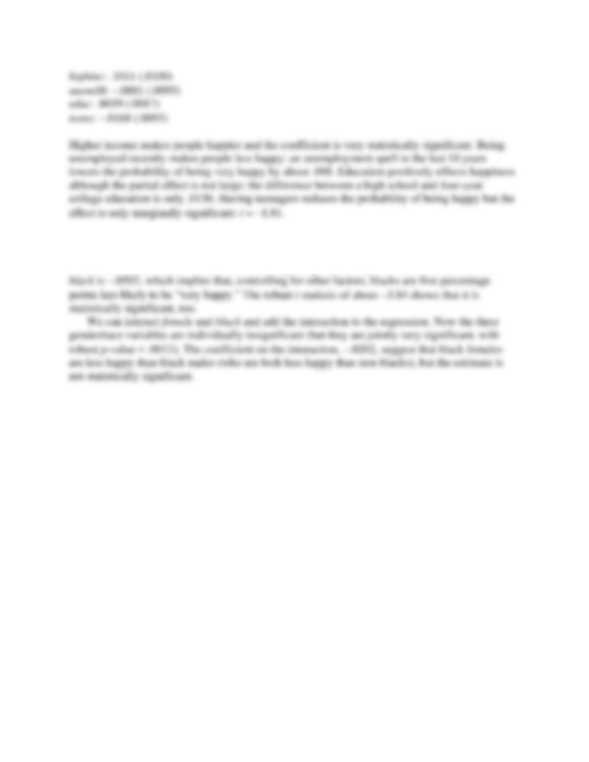
(v) The coefficients (robust ses) of the four new controls in part (iv) are
171
(vi) In this data set there is a gender variable and an indicator for whether the respondent is
black. I first just included female and black as explanatory variables. The coefficient on female is
small, .0022 (robust se = .0094) and statistically insignificant. By contrast, the coefficient on