Economics Chapter 13 One Factor Affecting The Sacrifice Ratio The

CHAPTER 13: UNEMPLOYMENT AND INFLATION

LEARNING OBJECTIVES

I. Goals of Part IV: Macroeconomic Policy: Its Environment and Institutions

A. How macroeconomic policy works and how it can best be used

1. Unemployment and inflation (this chapter)

II. Goals of Chapter 13

A. Why study unemployment and inflation together?

1. The most important macroeconomic problems

TEACHING NOTES

I. Unemployment and Inflation: Is There a Trade-off? (Sec. 13.1)

A. Many people think there is a trade off between inflation and unemployment

1. The idea originated in 1958 when A.W. Phillips showed a negative

relationship between unemployment and nominal wage growth in

Britain

2. Since then economists have looked at the relationship between

B. The expectations-augmented Phillips curve

1. Friedman and Phelps: The cyclical unemployment rate (the difference

between actual and natural unemployment rates) depends only on

unanticipated inflation (the difference between actual and expected

inflation)

Analytical Problem 3 looks at similar analysis in a Keynesian model.

Unemployment and Inflation 251

a. First case: anticipated increase in money supply (Fig. 13.1: like

text Fig. 13.3)

b. (1) AD shifts right and SRAS shifts left, with no misperceptions

(1) AD expected to shift right to AD2, old (money supply

expected to rise 10%), but unexpectedly money supply

rises 15%, so AD shifts further right to AD2 new

(2) SRAS shifts left based on expected 10% rise in money

supply

Numerical Problems 2 and 4 and Analytical Problem 2 look at the misperceptions model

and how it generates behaviour like the Phillips curve

Numerical Problem 1 uses the expectations-augmented Phillips curve.

C. The shifting Phillips curve

1. The Phillips curve shows the relationship between unemployment and

252 Chapter 13

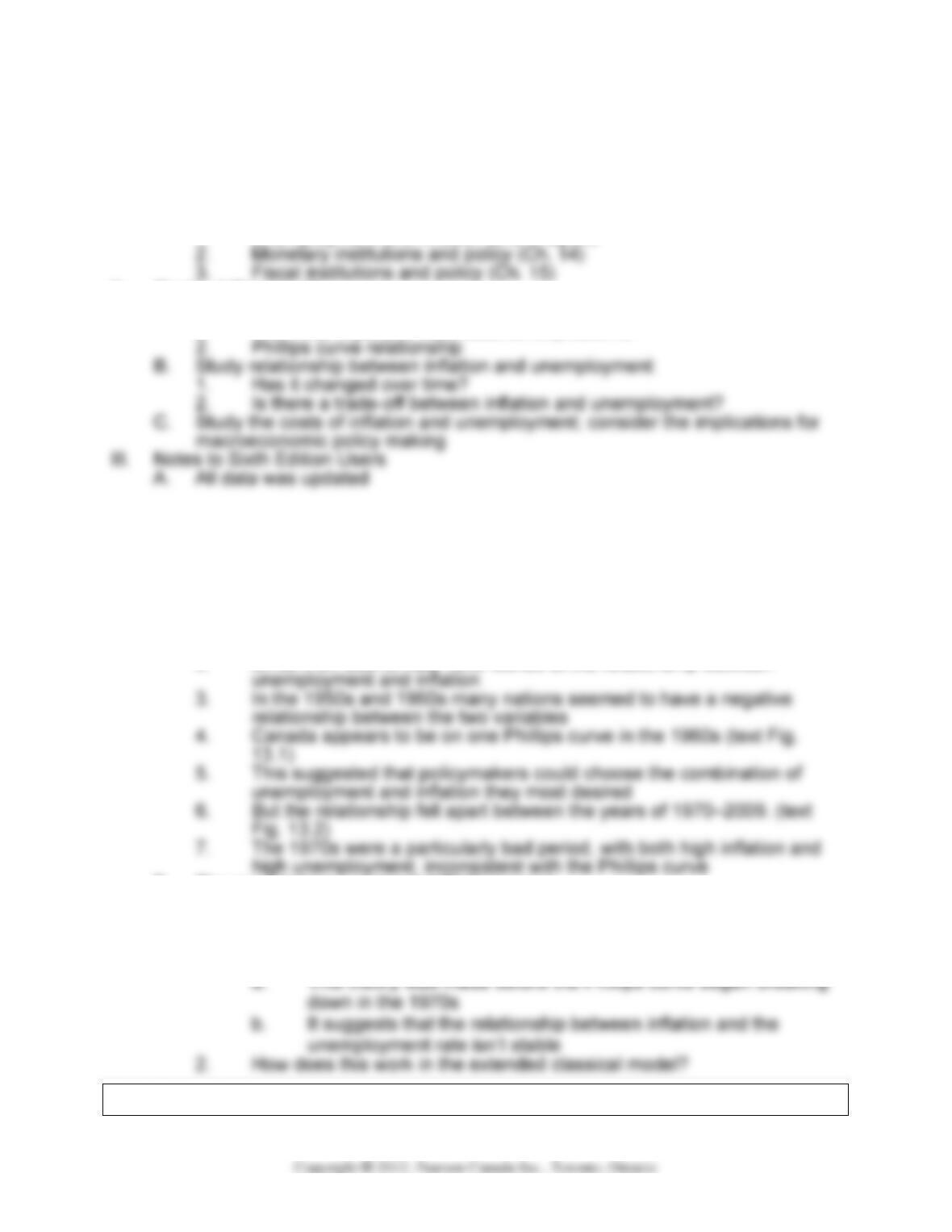
2. Changes in the expected rate of inflation (Fig. 13.3; like text Fig. 13.5)

a. For a given expected

rate of inflation, the

Phillips curve shows

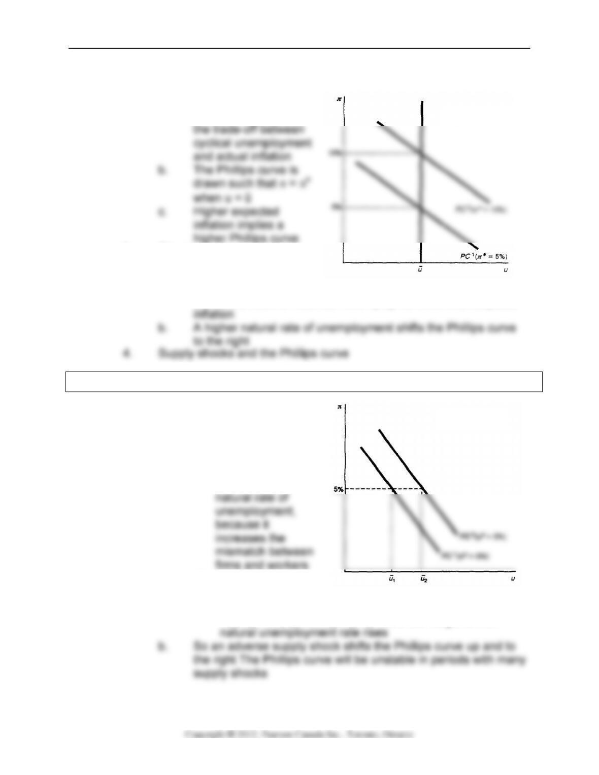
3. Changes in the natural rate

of unemployment (Fig. 13.4;

like text Fig. 13.6)

a. For a given natural rate of unemployment, the Phillips curve

shows the trade-off between unemployment and unanticipated

a. A supply shock

increases both

expected inflation and

the natural rate

(1) A supply shock in

the classical model

increases the

(2) A supply shock in

the Keynesian

model reduces the marginal product of labour and thus

reduces labour demand at the fixed real wage, so the

Analytical Problem 1 looks at possible ways to change the natural rate of unemployment.

Figure 13.4

Figure 13.3

Unemployment and Inflation 253

Numerical Problem 3 looks at the effects of an aggregate demand shock and an

aggregate supply shock on the Phillips curve.

5. The shifting Phillips curve in practice

a. Why did the original Phillips curve relationship apply to many

historical cases?

(1) The original relationship between inflation and

unemployment holds up as long as expected inflation and

b. Why did the Canadian Phillips curve disappear in the 1970s?

(1) Both the expected inflation rate and the natural rate of

unemployment varied considerably more in the 1970s than

they did in the 1960s

(2) Especially important were the oil price shocks of 1973–

D. Macroeconomic policy and the Phillips curve

1. Can the Phillips curve be exploited by policymakers? Can they choose

the optimal combination of unemployment and inflation?

a. Classical model: NO

(1) The unemployment rate returns to its natural level quickly,

as people’s expectations adjust

Policy Application

The theory of rational expectations explains why the Phillips curve trade-off appeared to

be stable for some time but failed when policymakers tried to exploit it. In the 1960s

254 Chapter 13

b. Keynesian model: YES, temporarily

(1) The expected rate of inflation in the Phillips curve is the

Theoretical Application

The Keynesian models of the early 1970s assumed that people formed adaptive

expectations, that is, that expected inflation depended only on past inflation, so

πet = f(πt-1, πt-2, …).

According to rational expectations theory, however, people base their inflation

expectations on an economic model in which inflation depends on other variables, such

2. A Closer Look 13.1: The Lucas critique

a. When the rules of the game change, behaviour changes

b. For example, if batters in baseball were called out after two

strikes instead of three, they’d swing more often when they have

one strike than they do now

Theoretical Application

The implications of the Lucas critique for future work on macroeconomics and business

cycles were spelled out by Robert Lucas and Tom Sargent in their article, “After

Keynesian Macroeconomics,” Federal Reserve Bank of Minneapolis Quarterly Review,

Spring 1979, pp. 1–16.

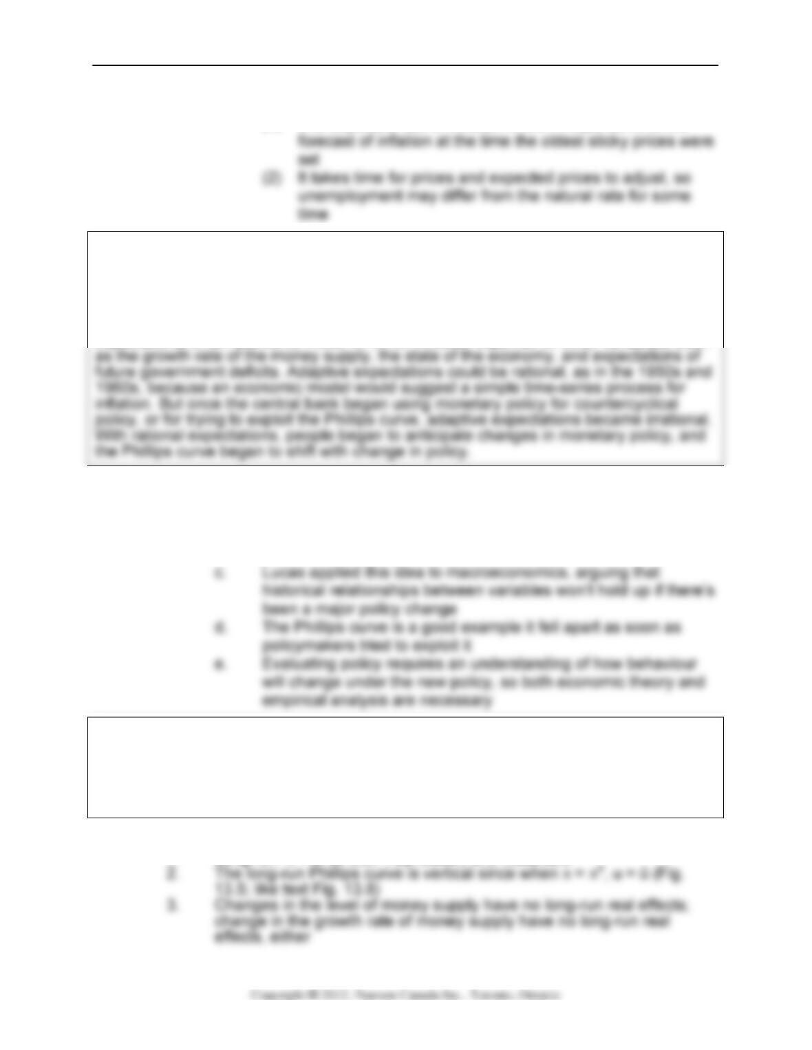
E. The long-run Phillips curve

1. Long run: u = ū for both Keynesians and classicals

Unemployment and Inflation 255

II. The Problem of Unemployment (Sec. 13.2)

A. The costs of unemployment

1. Loss in output from idle resources

a. Workers lose income

b. Society pays for unemployment benefits and makes up lost tax

2. Personal or psychological cost to workers and their families

3. There are some offsetting factors

a. Unemployment leads to increased job search and acquiring new

B. The long-term behaviour of the unemployment rate

1. The changing natural rate

a. How do we calculate the natural rate of unemployment?

b. Burns’ estimates: 4.5% in the mid-1960s, rising to 8.5% in the

256 Chapter 13

(a) Their unemployment rates are higher because of

discrimination, lower educational attainment,

(2) Technological change

(a) Technological changes have reduced the demand for

(3) Hysteresis in unemployment

(a) Hysteresis: The natural rate of unemployment rises

as the actual unemployment rate rises

(b) Caused partly by deteriorating skills of the

unemployed, which increases the mismatch problem

exceed market-clearing levels

(4) Changes in Unemployment Insurance (EI) legislation

Data Application

A readable series of papers on the natural rate of unemployment appeared in the Winter

1997 issue of the Journal of Economic Perspectives. The results are somewhat

negative: a number of authors argue that uncertainty about the value of the natural rate

means that it is of no use in guiding policy.

C. Policies to reduce the natural rate of unemployment

1. Government support for job training and worker relocation

2. Increased labour market flexibility

a. Regulations (like minimum wages, working conditions, fringe

3. Unemployment insurance reform

a. Unemployment insurance increases the time workers spend

Unemployment and Inflation 257

4. A high-pressure economy?

a. Using expansionary monetary and fiscal policies to create a

high-pressure economy could reduce the natural rate of

III. The Problem of Inflation (Sec. 13.3)

A. The costs of inflation

1. Perfectly anticipated inflation

a. No effects if all prices and wages keep up with inflation

Policy Application

Shoe-leather costs are generated by people’s attempt to reduce how much cash they

hold. Implicitly, inflation is like a tax on people’s cash holdings, because the government

buys things with newly printed money (just like it could if it collected taxes to pay for

them) and people who hold cash lose purchasing power (just as if their money was

taxed). Some economists have gone so far as to suggest that using the inflation tax is

beneficial to the economy, because much of the burden is borne by people in the

underground economy and foreigners who use US dollars. See S. Rao Aiyagari,

“Deflating the Case for Zero Inflation,” Federal Reserve Bank of Minneapolis Quarterly

Review, Summer 1990.

d. Menu costs: the costs of changing prices (but technology may

Analytical Problem 4 looks at the costs of anticipated and unanticipated inflation in a

cashless society.

2. Unanticipated inflation (π – πe)

a. Realized real returns differ from expected real returns

(1) Expected r = i – πe

258 Chapter 13

Data Application

Since the inflation of the mid-1970s was a surprise to people, it led to a large transfer of

wealth. The biggest winners in the 1970s were homeowners who owned land (which

d. So people want to avoid risk of unanticipated inflation

(1) They spend resources to forecast inflation

(2) A Closer Look 13.2: Indexed contracts

(a) People could use indexed contracts to avoid the risk

of transferring wealth because of unanticipated

inflation

with high inflation

e. Loss of valuable signals provided by prices

Data Application

For a review of the empirical evidence on the costs of inflation, see the article by John

Driftill, Grayham E. Mizon, and Alistair Ulph, “Costs of Inflation,” in B. M. Friedman and

F. H. Hahn, eds., Handbook of Monetary Economics, vol. II, Amsterdam: Elsevier

Science Publishers, 1990, pp. 1014–1066.

3. The costs of hyperinflation

a. Hyperinflation is a very high, sustained inflation (for example,

50% or more per month)

(1) Hungary in August 1945 had inflation of 19,800% per

month

Unemployment and Inflation 259

Data Application

There are many wonderful stories one can tell to illustrate the problems that arise in

hyperinflations. For example, there’s the story about the person who goes to the bank

with a wheelbarrow full of money, but can’t get the wheelbarrow through the bank’s

Policy Application

Given the costs of inflation and the vertical long-run Phillips curve, what is the optimal

rate of inflation? Some economists suggest that the optimal rate of inflation is zero or

even negative (so that the nominal rate of interest is zero). See the discussion by

Michelle R. Garfinkel, “What Is an ‘Acceptable’ Rate of Inflation? A Review of the

Issues,” Federal Reserve Bank of St. Louis Review, July/August 1989, pp. 3–15. The

B. Fighting inflation: The role of inflationary expectations

1. If rapid money growth causes inflation, why do central banks allow the

money supply to grow rapidly?

2. Disinflation is a reduction in the rate of inflation

a. But disinflations may lead to recessions

3. The costs of disinflation could be reduced if expected inflation fell at

the same time actual inflation fell

4. Rapid versus gradual disinflation

a. The classical prescription for disinflation is cold turkey—a rapid

and decisive reduction in money growth

260 Chapter 13

(c) The strategy might fail to alter inflation expectations,

because if the costs of the policy are high (because

the economy goes into recession), the government

will reverse the policy

Data Application

Tom Sargent (“The Ends of Four Big Inflations”) suggests that high rates of inflation

may be reduced quickly with little output loss if a country creates an independent central

b. The Keynesian prescription for disinflation is gradualism

(1) A gradual approach gives prices and wages time to adjust

to the disinflation

Policy Application

In the mid 1970s the Bank of Canada embarked on an attempt at gradualism, aiming to

bring clown inflation slowly by reducing the growth rate of M1. In face of financial

innovation and the supply shocks of 1979-80 however the policy was quite ineffective. It

was officially abandoned in 1982.

(2) Such a strategy will be politically sustainable because the

costs are low

5. A Closer Look 13.3: The sacrifice ratio

a. When unanticipated tight monetary and fiscal policies are used

to reduce inflation, they reduce output and employment for a

c. Ball studied the sacrifice ratios for many different disinflations

around the world in the 1960s, 1970s, and 1980s

(1) The sacrifice ratios varied substantially across countries,

from less than 1 to almost 3

Unemployment and Inflation 261

(a) Countries with slow wage adjustment (for example,

because of heavy government regulation of the labour

market) have higher sacrifice ratios

Data Application

A version of Bali’s article that is accessible to students is “How Costly Is Disinflation?

The Historical Evidence,” Federal Reserve Bank of Philadelphia Business Review,

November/December 1993, pp. 17–28.

6. Wage and price controls

a. Pro: Controls would hold down inflation, thus lowering expected

inflation and reducing the costs of disinflation

b. Con: Controls lead to shortages and inefficiency; once controls

Analytical Problem 5 looks at what happens if the government uses wage and price

controls, but continues to use expansionary monetary policy.

d. Application: The Nixon and Trudeau wage-price controls

(1) US price controls from August 1971 to April 1974

(2) Shortages developed in many products

(3) Gordon’s study suggested that the controls reduced

inflation when they were in effect, but prices returned to

(5) The Canadian experience of price controls between 1975–

1978 seems to have been more successful, reducing

inflation by about 3% per year and having little evidence of

262 Chapter 13

7. Credibility and reputation

a. Key determinant of the costs of disinflation: how quickly

expected inflation adjusts

ADDITIONAL ISSUES FOR CLASSROOM DISCUSSION

1. Additional Costs of Anticipated Inflation

The interaction of the tax system with inflation. Most countries’ tax systems are not

perfectly indexed for inflation. They impose taxes on nominal, not real, returns on

investments (bonds and stocks), which distorts the prices on those assets. Also, capital

gains are taxed in nominal terms, so investors may pay a big tax on assets whose value

hasn’t even increased in real terms. Eytan Sheshinski, in “Treatment of Capital Income

in Recent Tax Reforms and the Cost of Capital in Industrialized Countries,” in Larry

The mortgage tilt problem. Mortgage loans are most often made at fixed rates for long

terms. When inflation is positive, the constant nominal payment over time is much

higher in real terms early in the life of the loan, and lower in real terms later in the life of

the loan, because of a higher price level. This means that the burden of paying the loan

is high when households are younger. So if the households are liquidity constrained,

they may not be able to afford to buy a home as early as they could if there was no

inflation.

Here’s a numerical example. Consider a $100 000, 30-year mortgage. In case A

inflation is 0% and the nominal interest rate is 5%. The monthly payment is $540, the

Unemployment and Inflation 263

2. Can Unemployment Help Workers and the Economy?

If an unemployed worker always accepted the first job offered, unemployment would

decrease in the short run. However, such a practice is likely to reduce output and to

lead to more frequent periods of unemployment over several years. Accepting the first

ANSWERS TO TEXTBOOK PROBLEMS

Review Questions

1. The Phillips curve is an empirical negative relationship between inflation and

2. In the traditional Phillips curve, inflation itself is related to the unemployment rate.

In the expectations-augmented Phillips curve, it is unanticipated inflation (the

3. In the early 1960s the rate of inflation was fairly low (about 1% to 2%), and it didn’t

vary much from year to year. But supply shocks hit the economy in both the mid-

and the late-1970s, causing a rise in expected inflation and an upward shift in the

4. Both classical and Keynesian economists agree that unanticipated events cause

unanticipated inflation and so cause the unemployment rate to deviate from its full-

employment (or natural) rate. Classical economists stress that the economy

adjusts very quickly to unanticipated events and, as a result, they believe that the

264 Chapter 13

5. The natural rate of unemployment is the rate of unemployment that exists when

output is at its full-employment level. This occurs when the only unemployment is

frictional and structural, not cyclical. The natural rate is crucial in understanding the

Phillips curve.

6. Two costs of anticipated inflation are shoe-leather costs and menu costs. Two

costs of unanticipated inflation are transfers of wealth and confusion of price

signals.

7. The greatest potential cost of disinflation is that it may cause a recession. This

occurs because inflation may fall below expected inflation, causing the

8. One approach to disinflation is a cold turkey strategy. It has the advantage of

reducing inflation quickly, but it may have high costs from increasing

Numerical Problems

1. Since the natural rate of unemployment is 0.06, π = πe – 2(u – 0.06), so u – 0.06 =

0.5(πe – π) or u = 0.06 + 0.5(πe – π).

a. Year 1: u = 0.06 + 0.5(0.08 – 0.04) = 0.06 + 0.02 = 0.08. The unemployment

rate is 0.02 higher than the natural rate. The percentage that output falls short

Unemployment and Inflation 265

Year π πe u u–0.06 output shortfall

1 0.08 0.10 0.07 0.01 0.025

2. a. Equating aggregate demand to short-run aggregate supply gives: 300 + 10(M /

P) = 500 + P – Pe, or 300 + (10 × 1000 / P) = 500 + P – 50, or 10 000 / P = 150

b. When the nominal money supply increases unexpectedly to 1260, we again

equate aggregate demand to short-run aggregate supply, which gives: 300 +

10(M/P) = 500 + P – Pe or 300 + (10 x 1260 / P) = 500 + P – 50, or 12 600 / P =

150 + P. Multiplying both sides of the equation by P and rearranging gives P2+

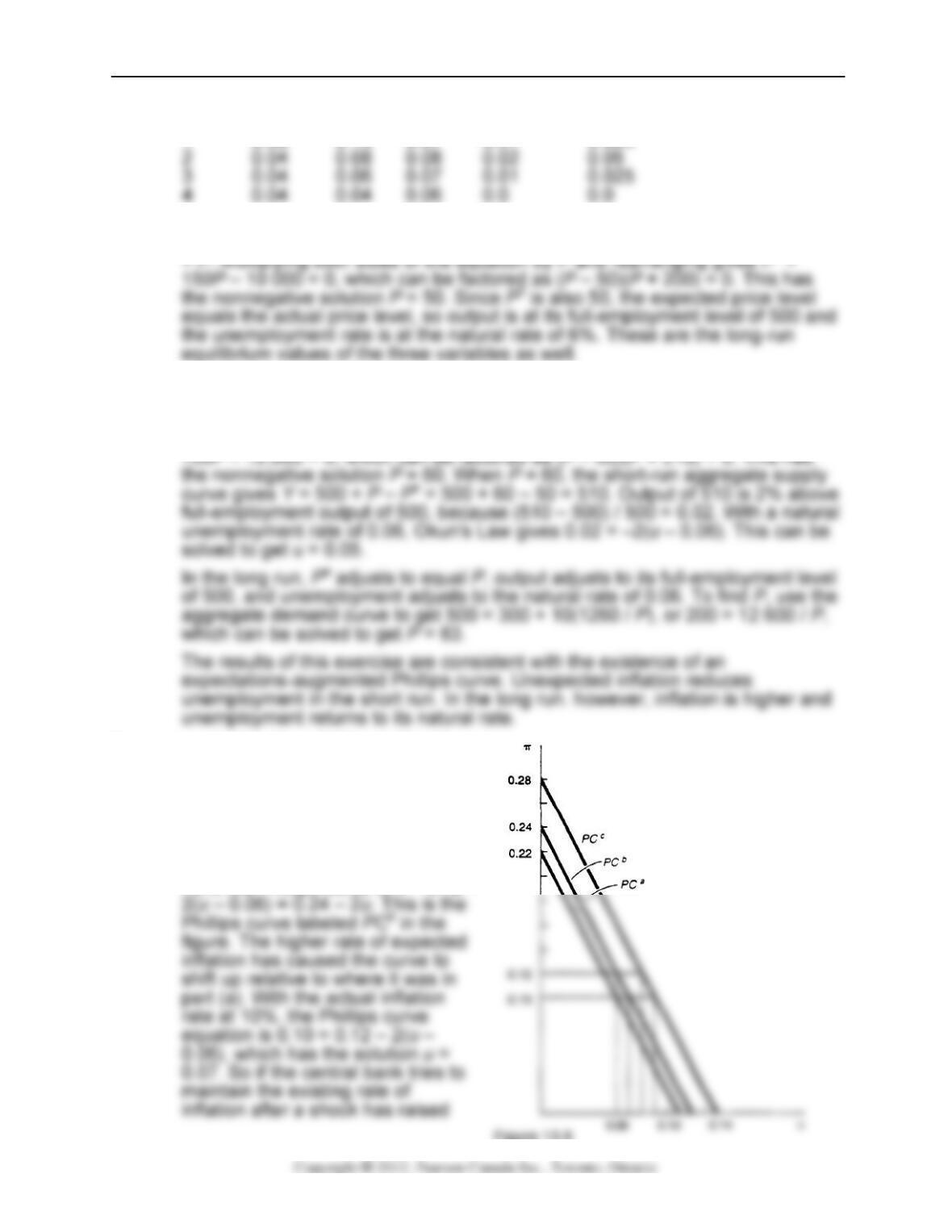
3. a. π = 0.10 – 2(u – 0.06) = 0.22 – 2u.

This is shown as the Phillips curve

labeled PCa in Fig. 13.6. If the

central bank keeps inflation at 0.10,

then u = 0.06, the natural rate of

unemployment.

b. With expected inflation rising to

12%, the Phillips curve is π = 0.12 –

Figure 13.6

266 Chapter 13

c. With the natural rate of unemployment rising to 0.08 at the same time that

expected inflation rises to 0.12, the Phillips curve equation is π = 0.12 – 2(u –

0.08) = 0.28 – 2u. This is the Phillips curve labeled PCc in the figure. The new

short-run Phillips curve is even higher than those for parts (a) and (b). With the

4. a. Beginning in long-run equilibrium, with M = 2000, output must be at its full-

employment level of 800 and the unemployment rate must be equal to the

natural rate of0.08. Using the values for Y and M in the AD curve, 800 = 400 +

5(2000/P), which gives P = 25. This is also the expected price level.

Unemployment and Inflation 267

Analytical Problems

1. a. The reduction in structural unemployment would reduce the natural rate of

unemployment and thus would shift both the expectations-augmented Phillips

2. The slope of the short-run aggregate supply curve will be much steeper in

economy B, because producers increase their output only a small amount in

response to an increase in price. But economy A’s short-run aggregate supply

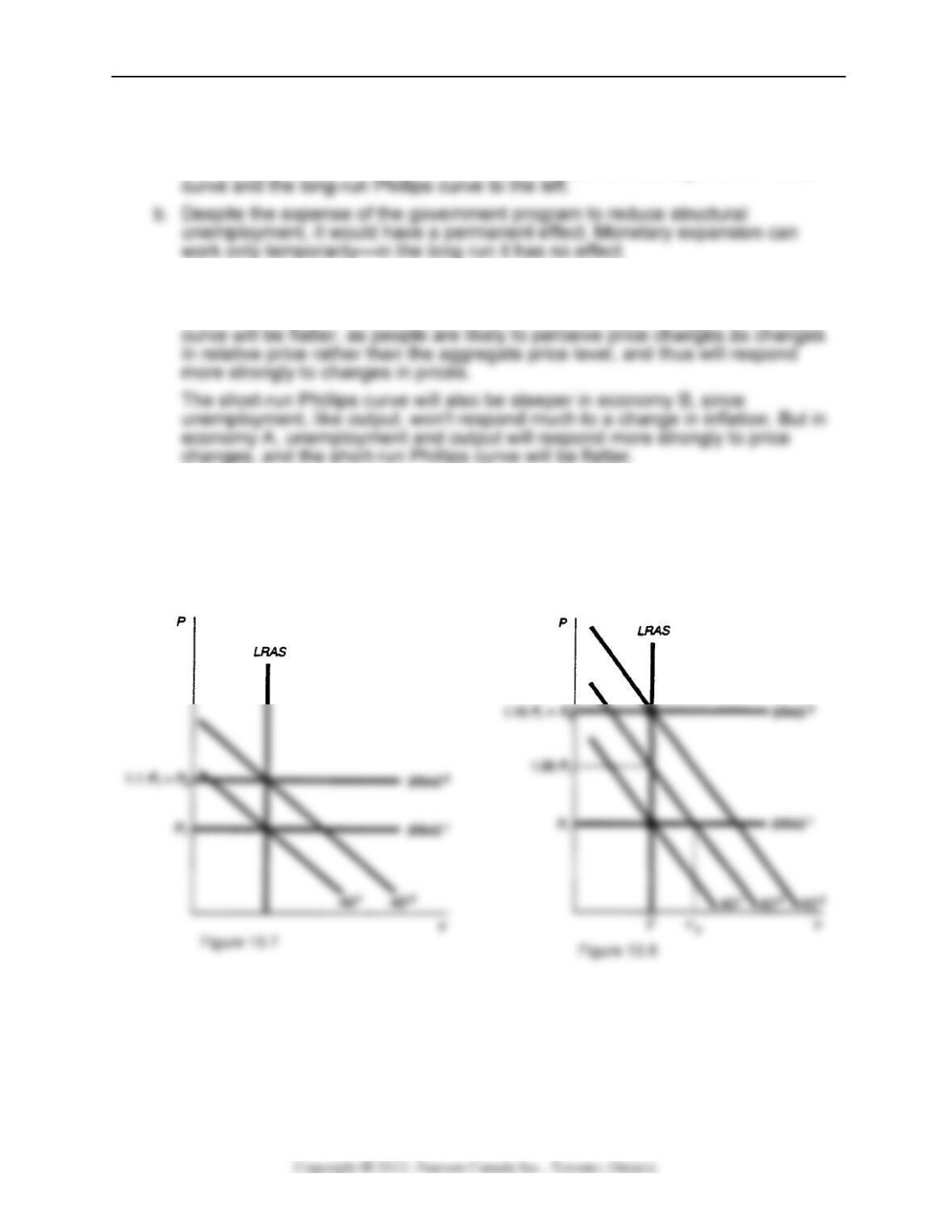
3. a. In Fig. 13.7, the SRAS curve shifts up 10% each year, as does the AD curve.

Unanticipated inflation is zero, as both actual and expected inflation are 10%.

The economy is at full employment, since firms set their prices to exactly match

the increase in the general price level.

268 Chapter 13

b. The surprise increase in the money supply at mid-year leads to a rise in output,

as shown in Fig. 13.8 by the shift of the AD curve from AD1 to AD2. Firms don’t

4. In the cashless society, there would be no shoe-leather costs, as there would be

no cash balances on which to economize. But menu costs would remain for

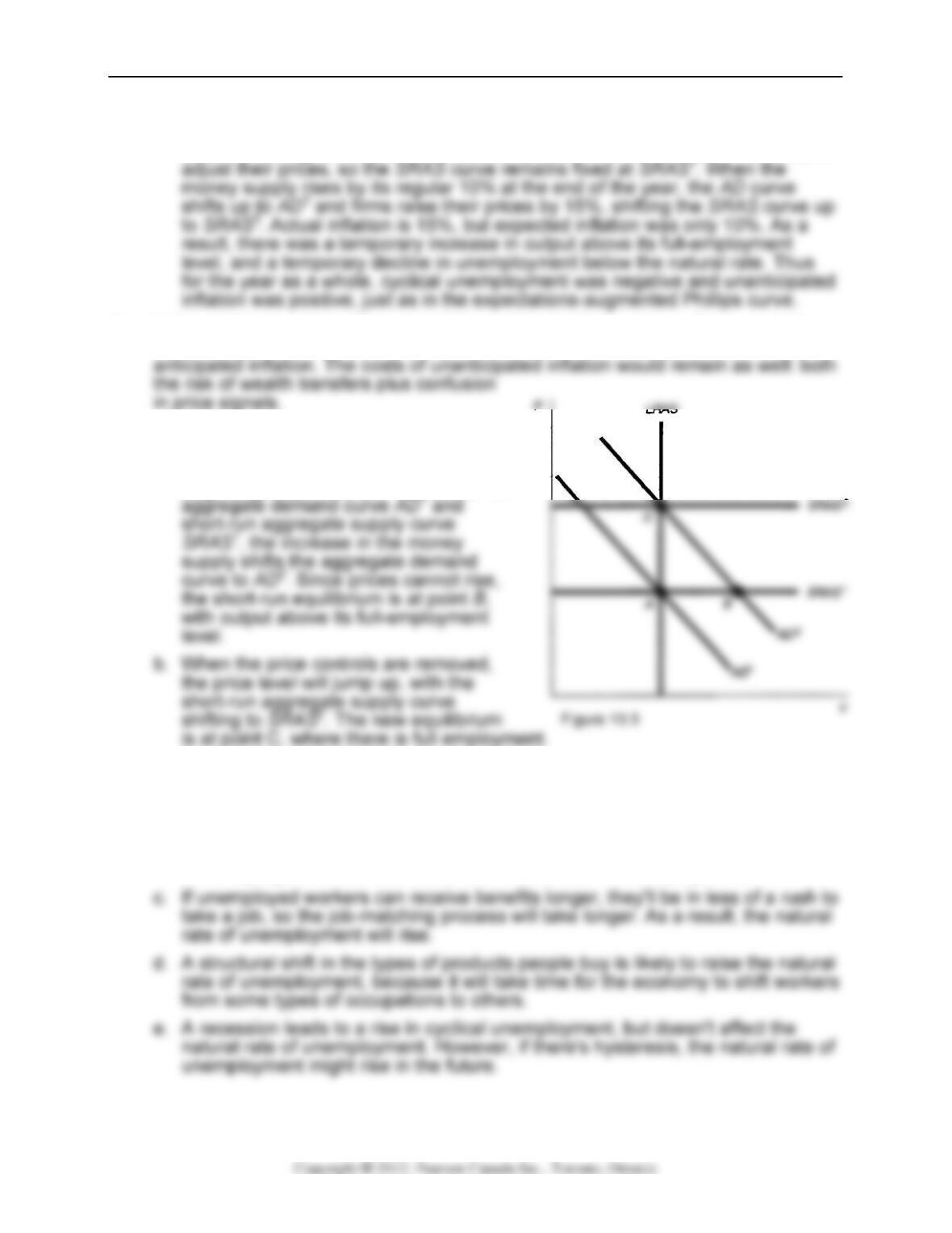
5. a. Figure 13.9 shows the effects of

increasing the money supply while

holding the price level constant.

Beginning at point A, the intersection of

6. a. A new law that prohibits people from seeking employment before age eighteen

is likely to reduce the natural rate of unemployment because teenagers have a

higher–than-average unemployment rate. With no teenagers allowed in the

labour force, the average unemployment rate would be lower.

b. A service that makes looking for a job easier is able to match people and jobs

more rapidly, which should reduce the natural rate of unemployment.