
CHAPTER 13 | Aggregate Demand and Aggregate Supply Analysis 313
Appendix
Macroeconomic Schools of Thought (pages 851–854)
Learning Objective: Compare macroeconomic schools of thought.
Macroeconomics became a separate field of economics in 1936, with the publication of John Maynard
Keynes’s book The General Theory of Employment, Interest and Money. The Keynesian revolution is
the name given to the widespread acceptance during the 1930s and 1940s of John Maynard Keynes’s
macroeconomic model. The aggregate demand and aggregate supply model developed by Keynes remains
The Monetarist Model
In the 1940s, Milton Friedman, an economist at the University of Chicago, developed the monetarist
model—also known as the neo-quantity theory of money model. Friedman argued that the Keynesian
The New Classical Model
New classical macroeconomics refers to the macroeconomic theories of Robert Lucas and others,
particularly the idea that workers and firms have rational expectations. This means that workers and firms
The Real Business Cycle Model
The real business cycle model is a macroeconomic model that focuses on real, rather than monetary,
causes of the business cycle. Proponents of this model argue that fluctuations in real GDP are caused by
temporary shocks to productivity.
The Austrian Model
The Austrian school of economics began in Austria in the late nineteenth century. The Austrian school is
best known for arguing the superiority of the market system over government planning.
314 CHAPTER 13 | Aggregate Demand and Aggregate Supply Analysis
Solutions to End-of-Chapter Exercises
13.1
Aggregate Demand
Learning Objective: Identify the determinants of aggregate demand and distinguish
between a movement along the aggregate demand curve and a shift of the curve.
Review Questions
1.1 The aggregate demand curve shows the relationship between the price level and the quantity of
real GDP demanded by households, firms, and the government. The short-run aggregate supply
1.2 The three reasons the aggregate demand curve slopes downward are the wealth effect, the
interest-rate effect, and the international-trade effect. The wealth effect refers to the effect that a
change in the price level has on wealth and, therefore, consumption. An increase in the price level
1.3 The aggregate demand curve shows the relationship between the price level and the quantity of
real GDP demanded by households, firms, and the government. The demand curve for an
individual product, such as apples, shows the relationship between the price of the individual
1.4 The variables that cause the aggregate demand curve to shift are interest rates, government
purchases, personal income taxes and business taxes, household expectations of future incomes,
firms’ expectations of the future profitability of investment spending, the growth rate of domestic
GDP relative to the growth rate of foreign GDP, and the exchange rate between the dollar and

CHAPTER 13 | Aggregate Demand and Aggregate Supply Analysis 315
investment spending and both will shift the AD curve to the left. An improvement in households’
expectations of future income will increase consumption and shift the AD curve to the right. An
Problems and Applications
1.5 a. An increase in the price level would cause a movement along the aggregate demand curve.
b. An increase in government purchases would cause the aggregate demand curve to shift to the
right.
1.6 The increase in stock prices relative to the price level, as measured by the consumer price index,
resulted in an increase in the real value of household wealth, which shifted the aggregate demand
curve to the right.
1.7 A movement from point A to point B along the aggregate demand curve would be caused by a
decrease in the price level. A movement from point A on aggregate demand curve AD1 to point C
1.8 You should disagree. The price level refers to average prices in the economy as a whole, so no
1.9 a. An increase in spending on machinery and equipment will shift the aggregate demand curve
to the right.
316 CHAPTER 13 | Aggregate Demand and Aggregate Supply Analysis
1.10 a. A “strong dollar” refers to an increase in the number of units of foreign currency—such as
the euro—that will be received in exchange for a dollar.
b. “Weak growth overseas” refers to slow, or negative, growth in output and income in foreign
1.11 U.S. net exports would increase if real GDP in the United States declined more than real GDP in
Canada, China, and other trading partners. With the larger decline in real GDP, U.S. imports
would decrease more than U.S. exports, and net exports would rise.
13.2
Aggregate Supply
Learning Objective: Identify the determinants of aggregate supply and distinguish
between a movement along the short-run aggregate supply curve and a shift of the
curve.
Review Questions
2.1 The long-run aggregate supply curve is vertical because in the long run changes in the price level
2.2 The variables that will cause the long-run aggregate supply to shift are: the size of the labor force,
2.3 As the prices of final goods and services rise, the prices of inputs usually rise more slowly. The
higher price level increases profits and the willingness of firms to supply more goods and
2.4 The variables that cause the short-run aggregate supply to shift are: the size of the labor force, the
size of the capital stock, productivity, the expected future price level, workers and firms adjusting
to having previously underestimated the price level, and the expected price of an important
CHAPTER 13 | Aggregate Demand and Aggregate Supply Analysis 317
Problems and Applications
2.5 a. A higher price level would cause a movement up along the long-run aggregate supply curve.
b. An increase in the labor force would cause the long-run aggregate supply curve to shift to the
2.6 You should disagree. The increase in aggregate supply, shown by the shift from SRAS1 to SRAS2,
2.7 A movement from point A to point B along the short-run aggregate supply curve would be caused
by an increase in the price level. A movement from point A on short-run aggregate supply curve
2.8 You should disagree. The labor force and the capital stock, along with technology, determine
potential GDP, but inflation expectations do not. Inflation expectations, however, do affect the
short-run aggregate supply of goods and services.
2.9 a. A higher price level would cause a movement up along the short-run aggregate supply curve.
b. An increase in what the price level is expected to be in the future would cause the short-run
aggregate supply curve to shift to the left.
2.10 a. A decrease in the expected future price level would match graph 3, where the short–run
aggregate supply curve shifts to the right, and the long-run aggregate supply curve does not
shift.
318 CHAPTER 13 | Aggregate Demand and Aggregate Supply Analysis
2.11 The reduction in the number of trucks and boxcars will increase transportation costs and shift the
short-run aggregate supply curve to the left. If shipping by boxcars continues to be a lower cost
2.12 Many economists believe that the main reason is that nominal wage cuts upset workers. As a
2.13 a. Firms are reluctant to lay off workers who have skills that the firms would have to replace
with new, less skilled workers after the recession ends and the demand for output rises.
Recruiting and training new workers to replace those who were previously laid off could be
2.14 Menu costs are costs to firms of changing prices. The widespread use of computers and the
Internet has made it less costly for firms to change prices and, therefore, has lowered menu costs.
13.3
Macroeconomic Equilibrium in the Long Run and the Short Run
Learning Objective: Use the aggregate demand and aggregate supply model to
illustrate the difference between short-run and long-run macroeconomic equilibrium.
Review Questions
3.1 When the economy is in long-run macroeconomic equilibrium, the short-run aggregate supply
curve and the aggregate demand curve intersect at a point on the long-run aggregate supply curve.
3.2 An adverse supply shock causes the short-run aggregate supply curve to shift to the left, resulting
3.3 2. The unemployment rate will rise in the short run as real GDP and income decline during the
recession. Rising unemployment and lower output will result in lower wages and prices.
CHAPTER 13 | Aggregate Demand and Aggregate Supply Analysis 319
Problems and Applications
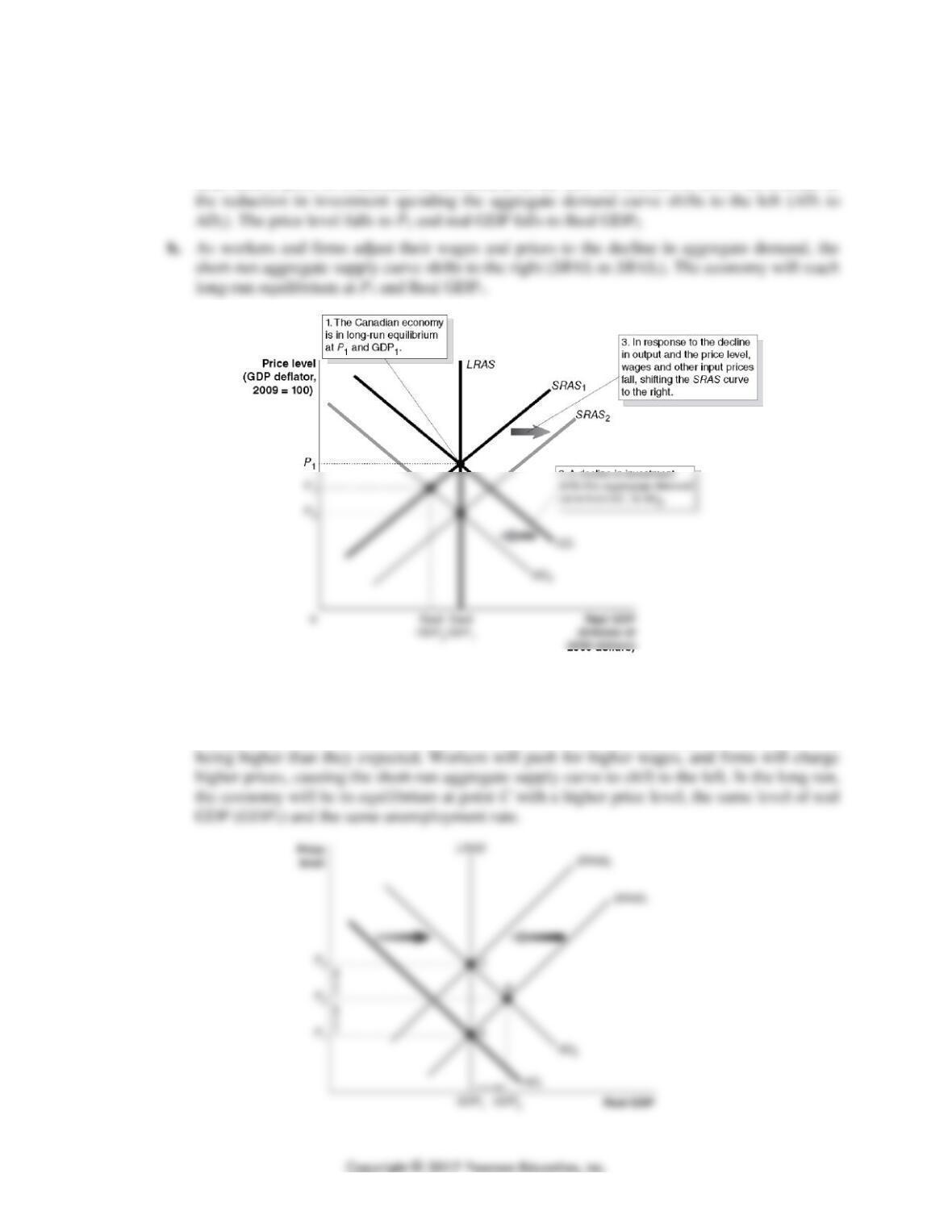
3.4 a. The graph below assumes that the Canadian economy was in long-run equilibrium (P1 and
Real GDP1) prior to a decrease in investment in the first six months of 2015. As a result of
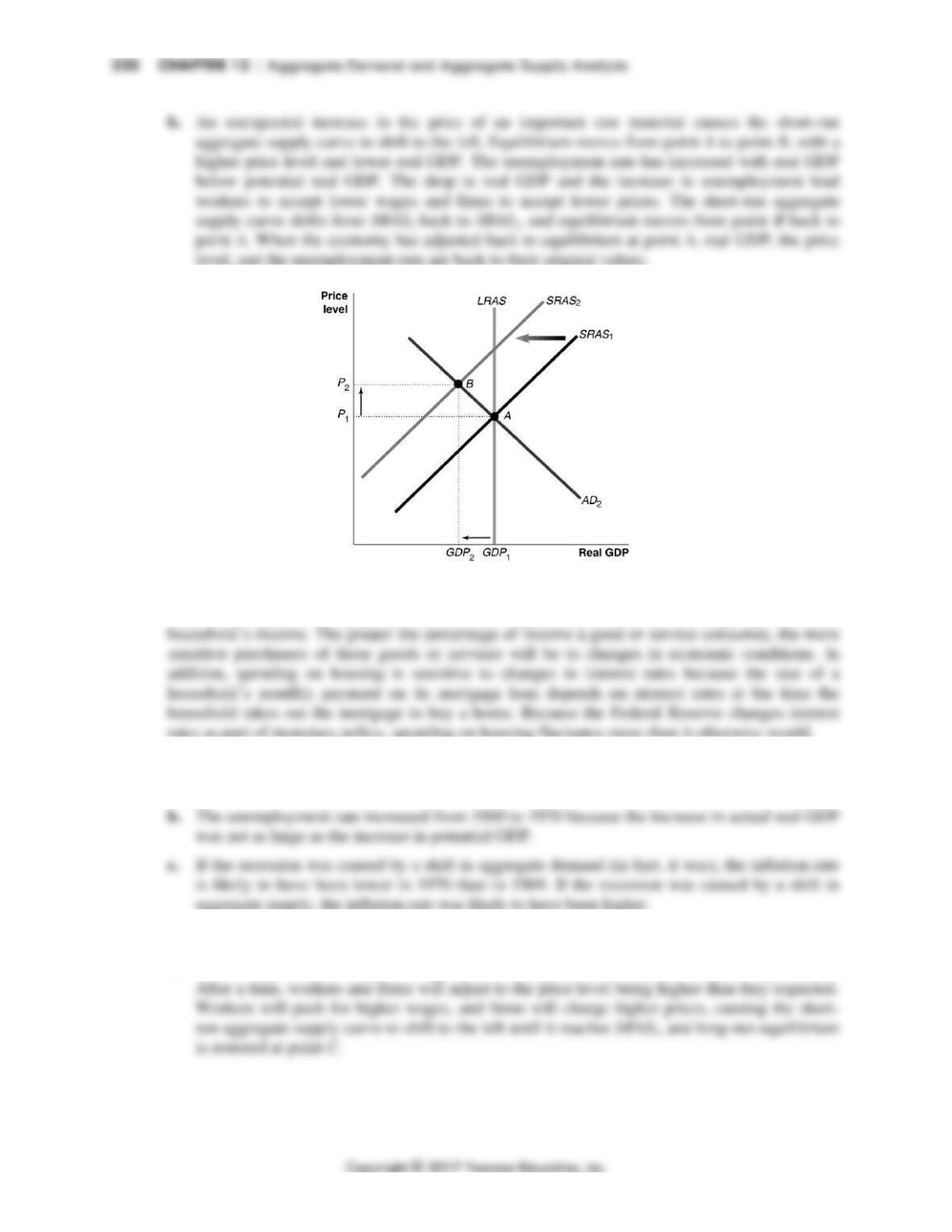
3.5 a. The large increase in the demand for U.S. exports shifts the aggregate demand curve to the
right, moving short-run equilibrium from point A to point B with a higher price level and
higher real GDP. The unemployment rate is lower because real GDP has increased with no
change in potential real GDP. Workers and firms will eventually adjust to the price level
3.6 Spending on housing is likely to fluctuate more than spending on consumer durables or spending
by firms on plant and equipment because housing usually consumes the largest portion of a
3.7 a. If firms operate beyond their normal capacity and structural and frictional unemployment
drop below their normal levels, then actual real GDP can be above potential GDP.
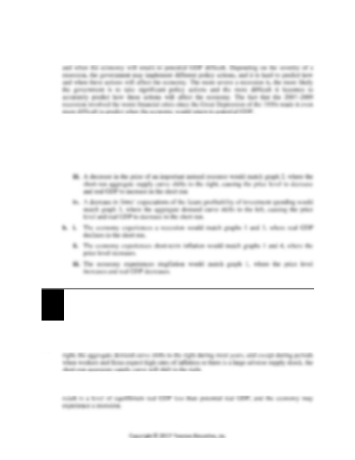
3.8 a. A and C represent long-run equilibrium points because they are on the LRAS curve.
b. Point D represents the short-run equilibrium and point C the eventual long-run equilibrium.
CHAPTER 13 | Aggregate Demand and Aggregate Supply Analysis 321
3.9 Many factors cause aggregate demand and aggregate supply to shift, and the difficulty of
determining which factors have changed, how much they have changed, and how those changes
will affect aggregate demand or aggregate supply make predictions of when a recession will end
3.10 a. i. An increase in the expected price level would match graph 1, where the short-run
aggregate supply curve shifts to the left, causing the price level to increase and real GDP
to decrease in the short run.
ii. An increase in households’ expectations of their future income would match graph 4,
where the aggregate demand curve shifts to the right, causing the price level and real
GDP to increase in the short run.
13.4
A Dynamic Aggregate Demand and Aggregate Supply Model
Learning Objective: Use the dynamic aggregate demand and aggregate supply model
to analyze macroeconomic conditions.
Review Questions
4.1 In the dynamic model, potential real GDP increases continually, shifting the LRAS curve to the
4.2 If aggregate demand increases more than potential real GDP increases, the economy will
experience inflation. If aggregate demand increases less than potential real GDP increases, the
322 CHAPTER 13 | Aggregate Demand and Aggregate Supply Analysis
4.3 The factors that brought on the recession of 2007–2009 were the collapse of the housing bubble,
the financial crisis, and the rapid increase in oil prices during 2008. The collapse of the housing
Problems and Applications
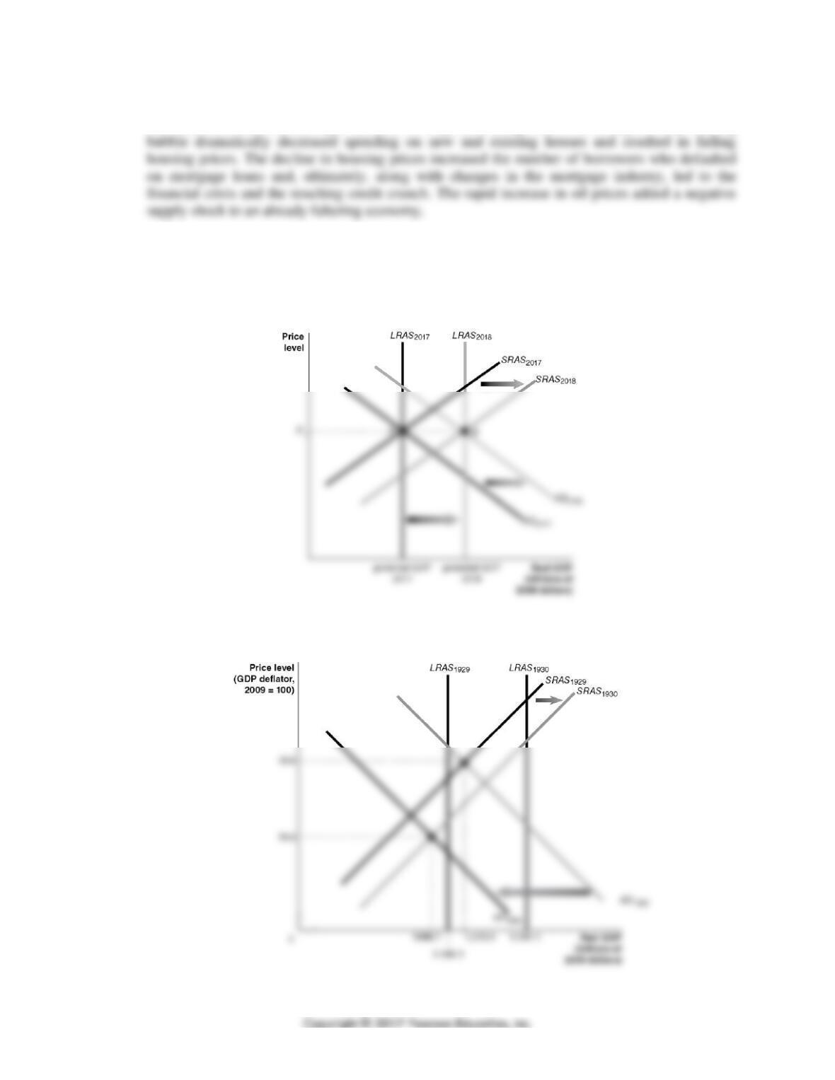
4.4 To move from potential GDP in 2017 to potential GDP in 2018 without inflation, aggregate
demand, long-run aggregate supply, and short-run aggregate supply must all increase—or, shift to
the right—by the same amount.
4.5 a. The price level fell during 1930, which it has not done for an entire year since the 1930s.
b.
CHAPTER 13 | Aggregate Demand and Aggregate Supply Analysis 323
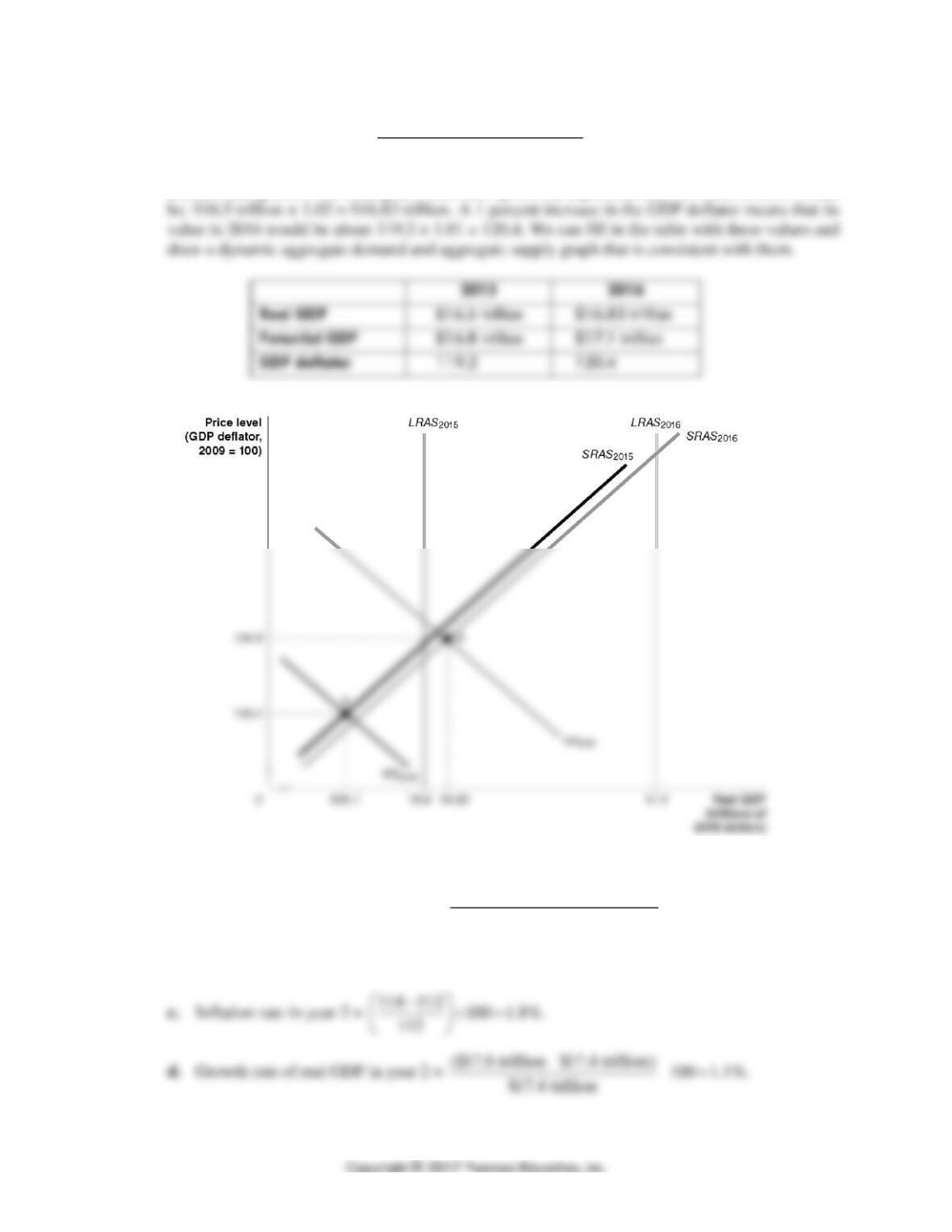
4.6 Potential GDP increases by
($17.1 trillion –$16.8 trillion)
$16.8 trillion ´100 =1.79%.
So, to be consistent
with the economists’ forecast, the value of real GDP would have to grow by more than this
amount during 2015. For example, if real GDP grows by 2 percent, then its value in 2016 would
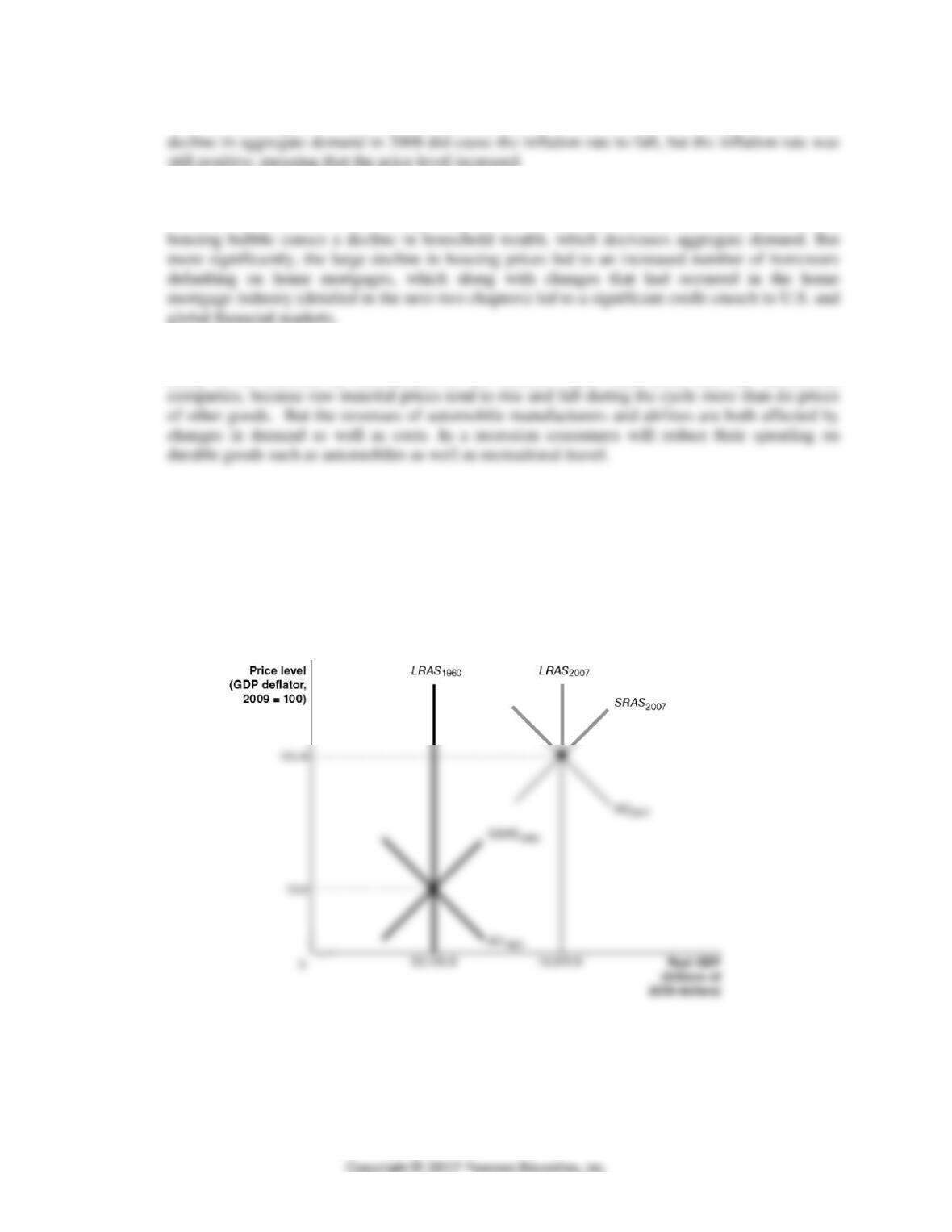
4.7 a. Growth rate of potential real GDP =
($17.8 trillion –$17.4 trillion)
$17.4 trillion ´100 =2.3%.
b. The unemployment rate will be higher in year 2 because the economy is below potential
GDP.
324 CHAPTER 13 | Aggregate Demand and Aggregate Supply Analysis
4.8 You should disagree because the statement confuses the inflation rate with the price level. The
4.9 The housing bubble refers to a rapid increase in prices in the housing market in the early 2000s,
followed by a decline in prices beginning in 2006 after they reached unsustainable levels. A
4.10 Firms such as Delta Air Lines whose costs are highly dependent on raw material prices are more
likely to be affected by fluctuations in the business cycle than firms like the automobile
Real-Time Data Exercises
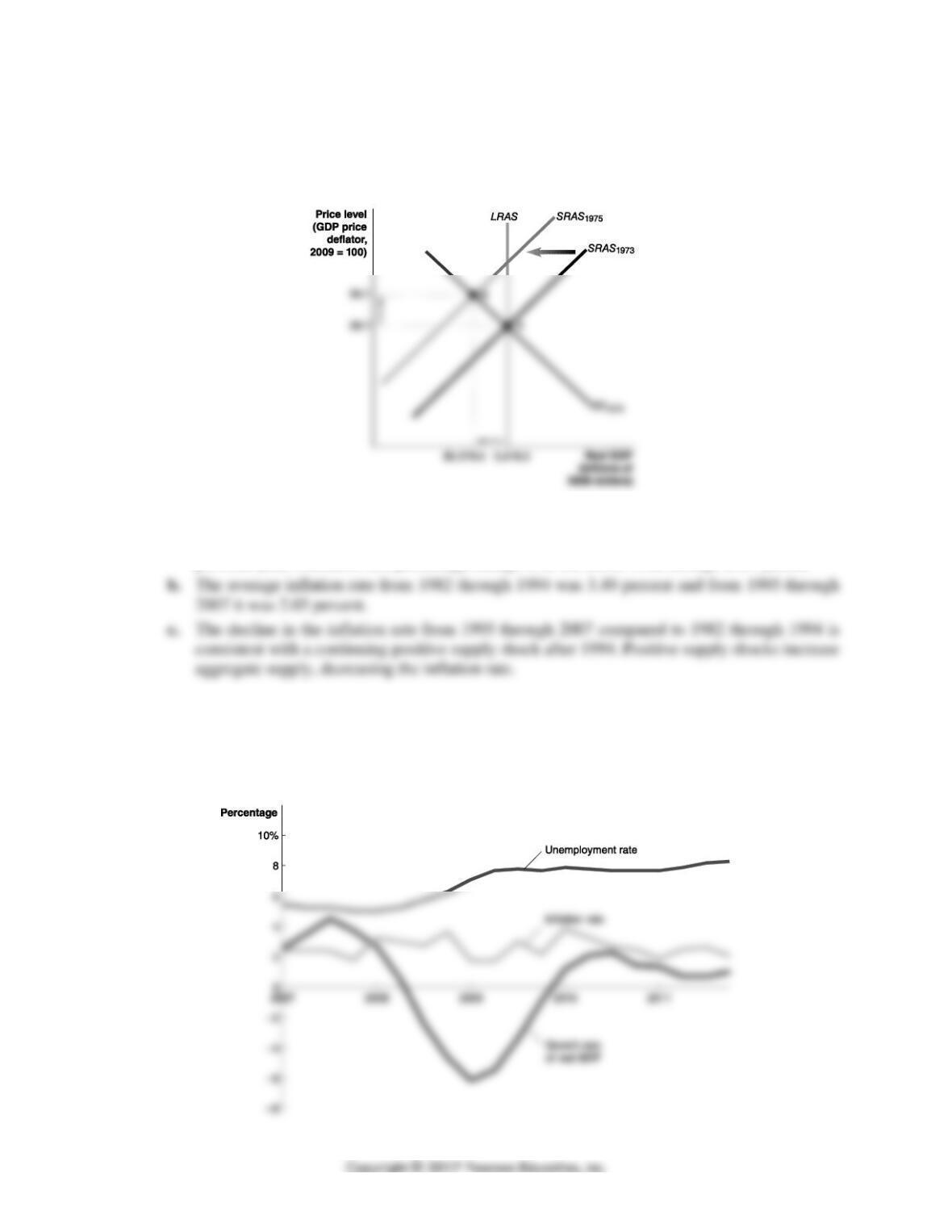
D13.1 a. The graph below shows the economy at equilibrium at potential GDP in 1960 and in 2007.
With real GDP rising from $3,105.8 billion in 1960 to $14,876.8 billion in 2007, the long-run
aggregate supply curve shifted to the right. With the GDP price deflator rising from 19.0 in
1960 to 105.8 in 2007, aggregate demand grew more than long-run aggregate supply.
CHAPTER 13 | Aggregate Demand and Aggregate Supply Analysis 325
b. Given that real GDP declined from $5,418.2 billion in 1973 to $5,379.5 billion in 1975 and
that the GDP price deflator rose from 28.7 in 1973 to 34.1 in 1975, the short-run aggregate
supply curve shifted to the left from 1973 to 1975. For simplicity, the graph below shows for
1975 only the shift to the left of the short-run aggregate supply curve.
D13.2 a. As indicated in the exercise, download monthly data on the personal consumption
expenditure price index and calculate the percentage change from the same month in the
previous year. Calculate this percentage change over the entire 1982 through 2007 period.
D13.3 a. Data used in the graph in part (b). Choose quarterly for the frequency of the unemployment rate.
b. The United Kingdom has had a similar experience to the United States since 2007. The
United Kingdom experienced a larger drop in real GDP in late 2008 and early 2009 and has
had slower growth in real GDP since 2009. From 2007 to 2012, the United Kingdom
experienced higher inflation and lower unemployment than the United States.