198
CHAPTER 13
Pricing in Input Markets
A. Summary
This chapter provides a brief introduction to supply and demand in input
markets. In order to make the analysis less abstract, most of the focus is on
labor markets though it might hold equally well for any other input market.
B. Lecture and Discussions Suggestions
The presentation of input demand in Chapter 13 includes two analytical con-
cepts that are especially difficult for students and these should be featured in
lectures. First, the output and substitution effects from a change in input pric-
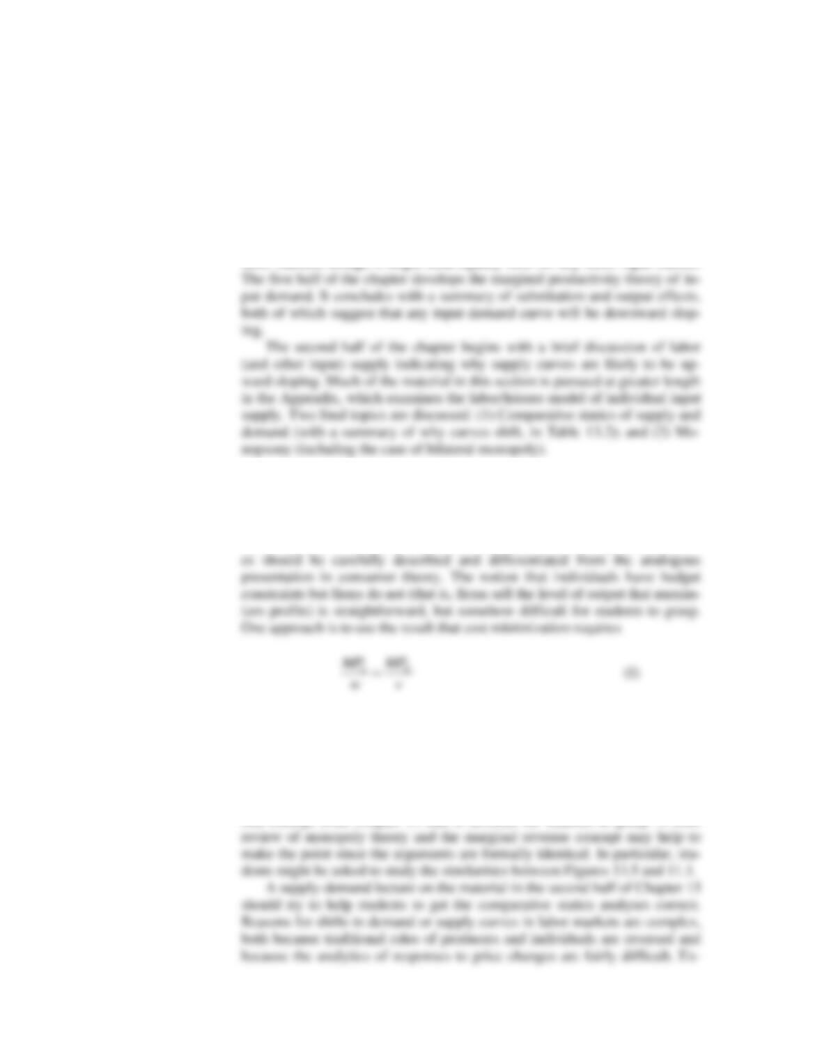
and note that this common ratio equals 1/MC. Changes in an input’s price,
therefore, prompts substitution effects from equation (1) and output effects
from changes in 1/MC (which must equal 1/MR for profit maximization).
Both of these changes imply input prices and levels of input use move in op-
posite directions.
Marginal expense (sometimes termed “marginal factor cost”) is the sec-
ond concept from Chapter 13 that is difficult for students to grasp. A brief
Chapter 15: Pricing in Input Markets
199
plaining in detail why each of the entries in Table 13.2 shifts the curves in
the directions indicated, though a dull exercise, may significantly aid stu-
dents’ understanding.
There is no end to potentially interesting discussion topics for the materi-
C. Glossary Entries in the Chapter and Appendix
• Bilateral Monopoly
• Income Effect of a Change in w
SOLUTIONS TO CHAPTER 13 PROBLEMS
13.1 a. With five workers, put each successively where its marginal product is greatest.
First worker goes to A, second goes to B, third goes to A, fourth goes to C, fifth
goes to A. Output = 21 + 8 + 5 = 34. MP of last worker is 4.
c. Marginal products of labor on the various farms are:
Workers MPA MPB MPC
1 10 8 5
13.2 For this problem, the production function is q = 10,000
L
and MPL = 5,000/
L
.
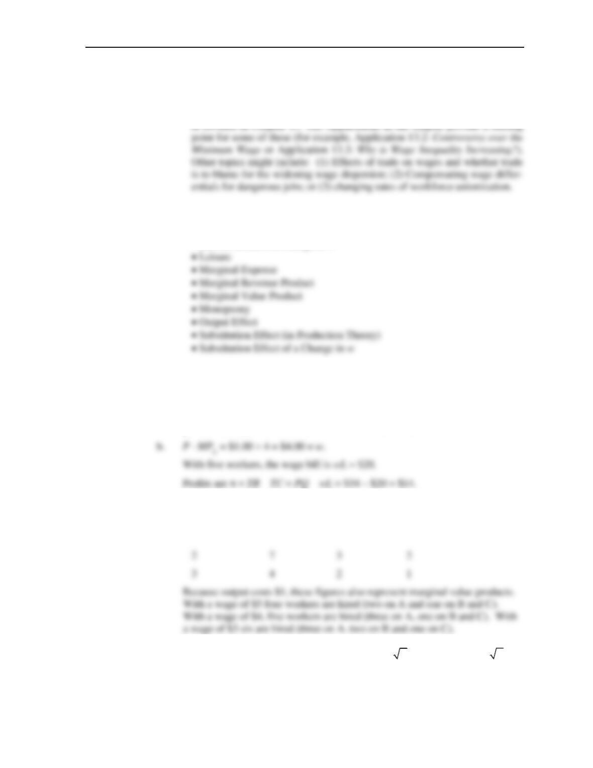
a. Since P = .01 here and the firm is a price taker, profit maximization requires
that
Chapter 15: Pricing in Input Markets
200
As these points suggest, this demand curve has a hyperbolic shape.
b. Assuming w = $10, the value of the marginal product is P 5,000/
L
;
If P = .10: 10 = 500/
L
:
L
L
L
= 50, q = 500,000
The graph shows the supply curve for licked envelopes.
13.3 a. w = v = $1, so K and L will be used in a one-to-one ratio.
Chapter 15: Pricing in Input Markets
201
b. Since P = 2, quantity demanded is Q = 400,000 – 100,000(2) = 200,000 pipe
q = 200 =
KL
= 4 so 200 workers are hired per firm, 200,000 by the indus-
try.
c. When w = $2 and v = $1, cost minimization requires
e. If output had stayed at q = 200, L = 200/
2
= 141.4 so total hiring would be
141,400. Reduction from 200,000 to 141,000 is the substitution effect. From
141,400 to 87,900 is the output effect.
13.4 Demand: L = –50w + 450. Supply: L = 100w.
a. Equilibrium can be found by setting quantity supplied equal to quantity de-
manded.
Chapter 15: Pricing in Input Markets
202
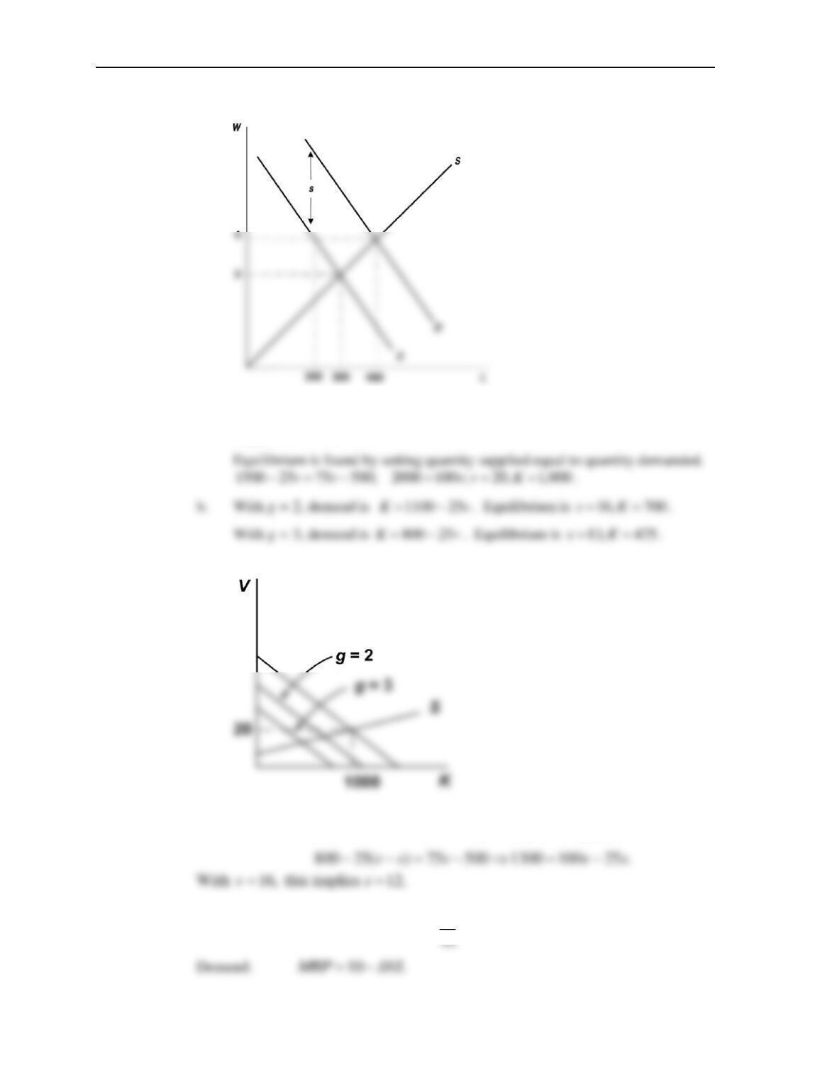
d. The graph shows these various equilbria in the labor market.
13.5 a. Demand:
1500 25Kv=−
Supply:
75 500Kv=−
c.
d. Need to restore the rental rate to
16.v=
Let s be the subsidy per car. Then
demand is
800 25( )K v s= − −
. Setting this equal to supply yields:
13.6 Supply: L = 100w
L
L
ME =
Chapter 15: Pricing in Input Markets
203
a. Hence, profit maximization requires
b. For perfectly competitive labor market MRPL = w in equilibrium. So from sup-
ply curve
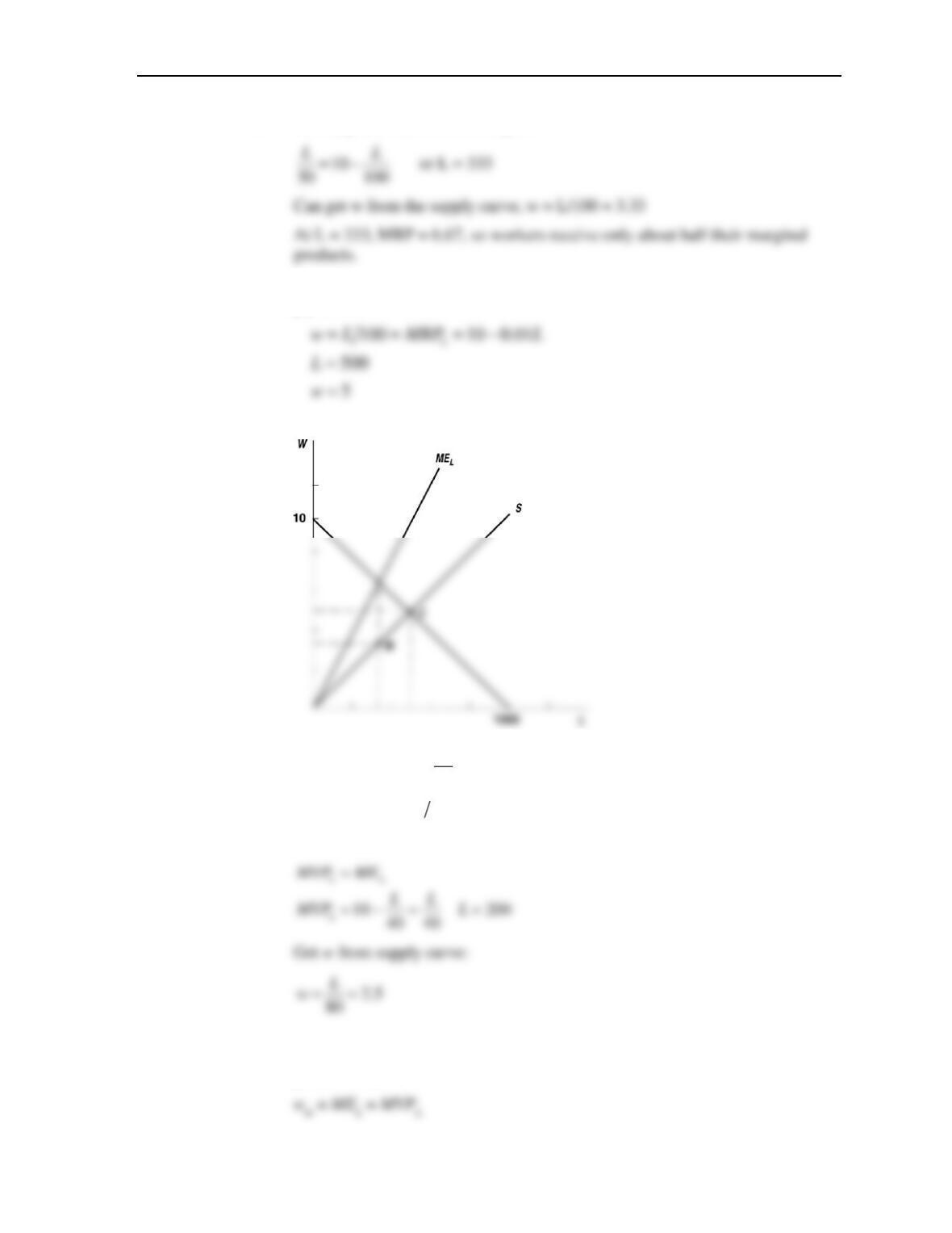
The graph shows both the monopsonistic (M) and competitive (C) equilibria.
13.7 Supply:
80 40
L
L
L w ME==
Demand:
10 40
L
MVP L=−
a. For monopsonist
b. For Carl, the marginal expense of labor now equals the minimum wage and in
equilibrium the marginal expense of labor will equal the marginal revenue
product of labor.
Chapter 15: Pricing in Input Markets
204
wm = $3.00.
Carl’s Demand Supply
Since quantity demanded exceeds quantity supplied. Carl will hire 240 work-
ers, with no unemployment. To study effects of minimum, try $3.33 and $4.00
wm = $3.33
Carl’s Demand Supply
Carl’s Demand Supply
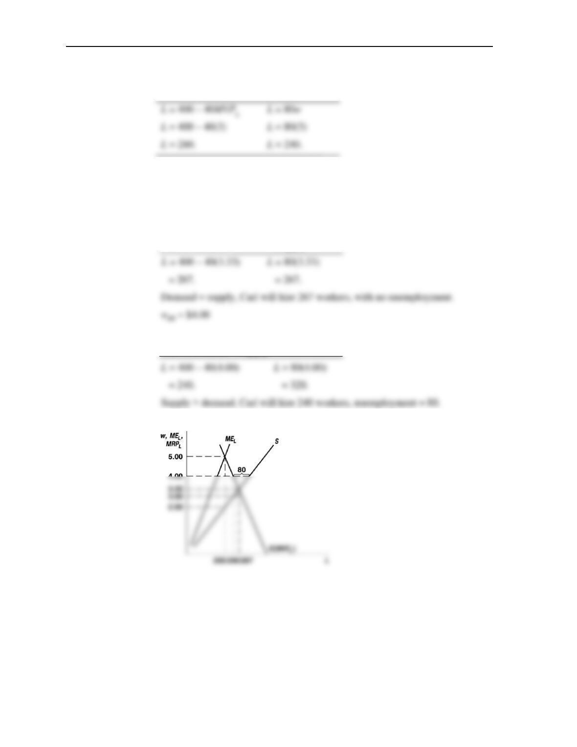
c. The graph shows these various responses to a minimum wage.
d. Under perfect competition, a minimum wage means higher wages but fewer
workers employed. Under monopsony, a minimum wage may result in higher
wages and more workers employed as shown by some of the cases studied in
part b.
13.8 Here marginal value product is $10 per hour:
Chapter 15: Pricing in Input Markets
205
MEm =
m/2 L
= 10 so Lm = 400, wm = 20/3 = 6.67.
13.9 a. Budget constraint: C = w(24 – H) + 10.
b. Due to Mrs. Smith’s preferences, she insists on spending half of potential earn-
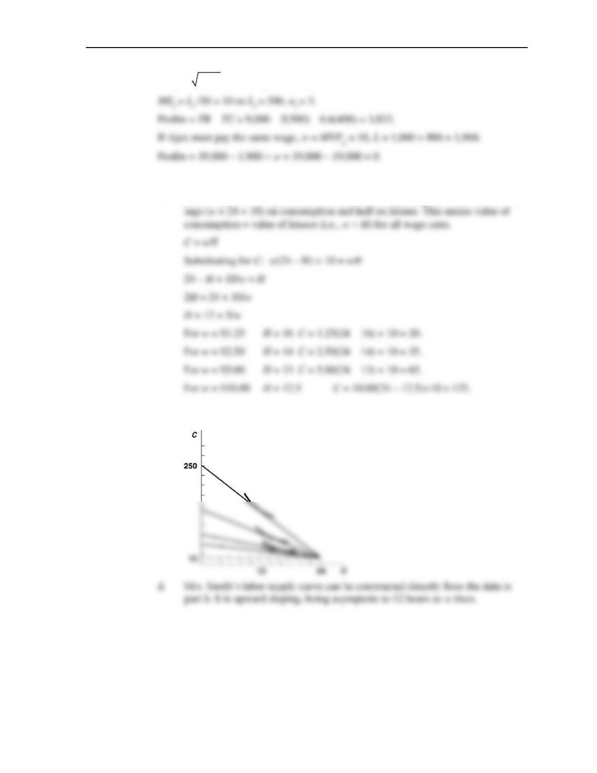
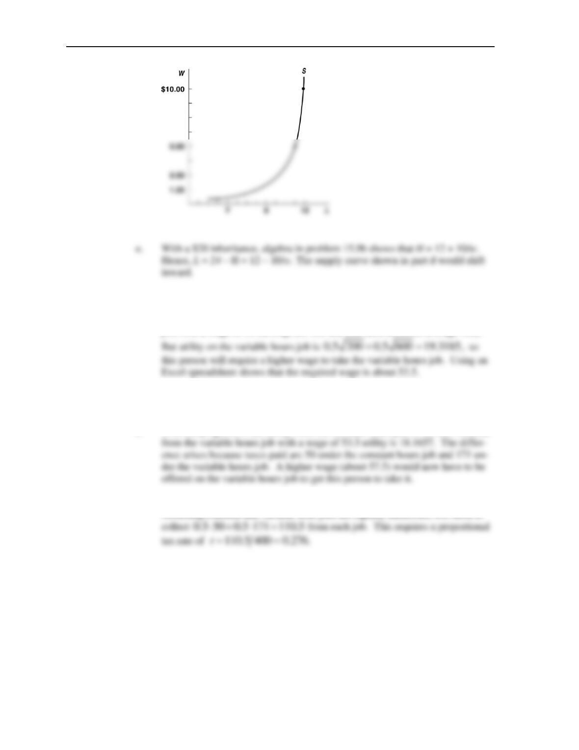
c. The graph shows Mrs. Smith’s changing choices as the wage rises. Hours of
leisure (H) fall toward 12 as w rises.
Chapter 15: Pricing in Input Markets
206
13.10 a. Earnings on 8 hour days are 400. Hence utility is 20. On the variable hours
job, with a wage of 50 earnings are 200 and 600 (and therefore average 400).
b. A proportional tax will not affect the utility calculation because the tax rate will
factor out of all of the expressions for utility.
c. With the progressive tax utility from the constant hours job is 18.7083 whereas
d. To answer this part one must assume something about the distribution of jobs.
Assuming constant and variable hour jobs are equally numerous, will need to