Chapter 13
Minimum Distance Estimation and
the Generalized Method of Moments
◼ Exercises
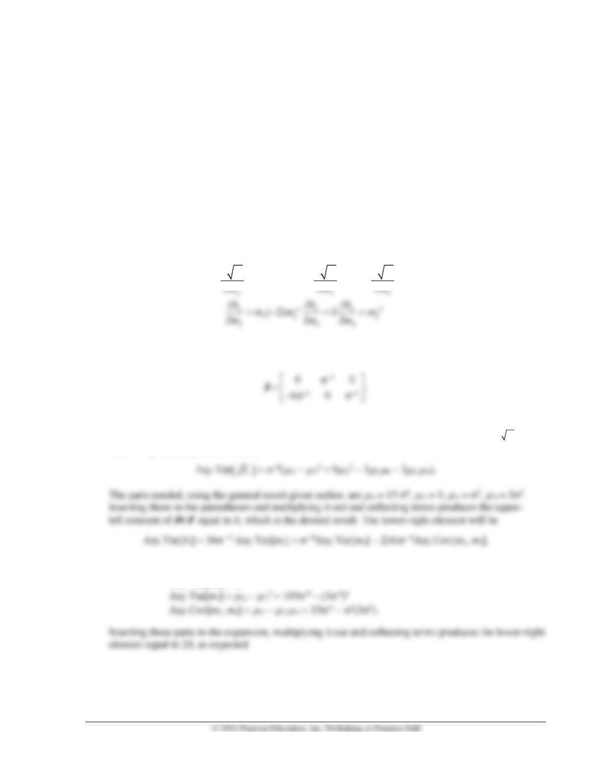
1. The elements of J are
−
= − = =
1 1 1
5/2 3/2
3 2 2
( 3/2) 0
b b b
m m m
Using the formula given for the moments, we obtain,
2 = 2,
3 = 0,
4 = 34. Insert these in the
derivatives above to obtain
Since the rows of J are orthogonal, we know that the off-diagonal term in JVJ will be zero, which
simplifies things a bit. Taking the parts directly, we can see that the asymptotic variance of
1
b
will
be −6 Asy.Var[m3], which will be
The needed parts are
Asy.Var[m2] = 24
112 Greene • Econometric Analysis, Seventh Edition
2. The necessary data are given in Example 13.5. The two moments are
1
m
= 31.278 and
2
m
= 1453.96.
Based on the theoretical results
1
m
= P/ and
2
m
= P(P + 1)/2, the solutions are P =
22
1 2 1
/( )
−
and =
−2
1 2 1
/( ).
Using the sample moments produces estimates P = 2.05682 and = 0.065759.
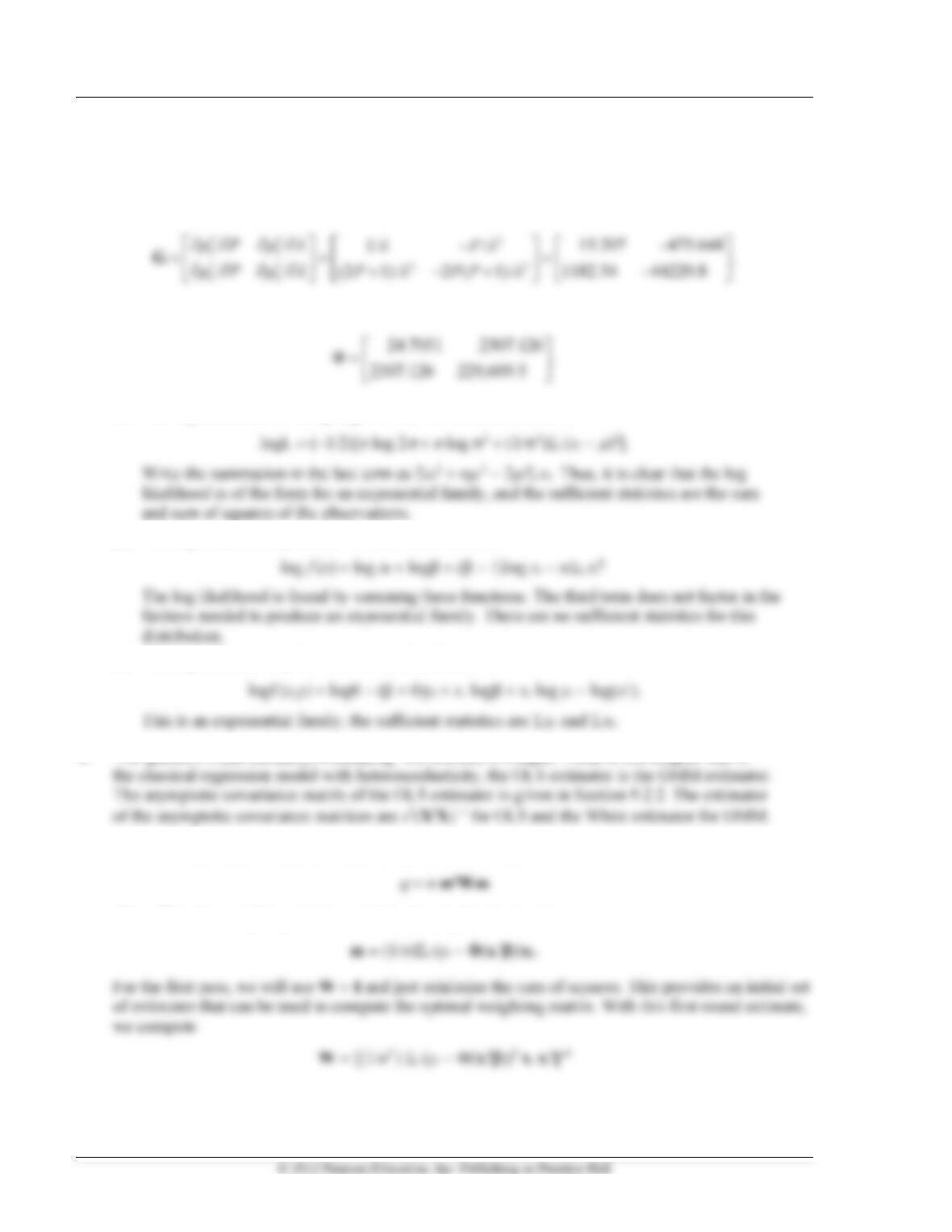
The matrix of derivatives is
The covariance matrix for the moments is given in Example 18.7;
3. (a) The log likelihood for sampling from the normal distribution is
(b) The log of the density for the Weibull distribution is
(c) The log of the density for the mixture distribution is
4. The question is (deliberately) misleading. We showed in Chapter 9 and in this chapter that in
5. The GMM estimator would be chosen to minimize the criterion
where W is the weighting matrix and m is the empirical moment,
Chapter 13 Minimum Distance Estimation and the Generalized Method of Moments 113
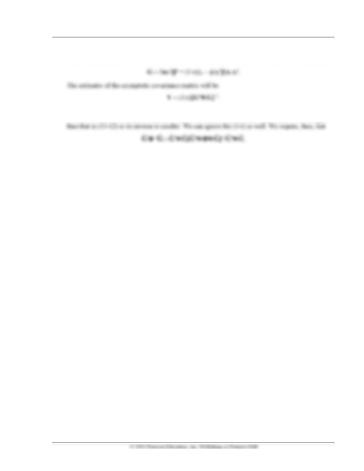
then return to the optimization problem to find the optimal estimator. The asymptotic covariance
matrix is computed from the first-order conditions for the optimization. The matrix of derivatives is
6. This is the comparison between (13-12) and (13-11). The proof can be done by comparing the
inverses of the two covariance matrices. Thus, if the claim is correct, the matrix in (13-11) is larger