285
CHAPTER 13
The Open Economy Revisited: The
Mundell–Fleming Model and the
Exchange–Rate Regime
Notes to the Instructor
Chapter Summary
Chapter 13 presents the Mundell–Fleming model of a small open economy in the short run.
Essentially, it is a synthesis of the IS–LM model and the small open economy model of Chapter
1. To introduce students to the distinction between fixed and floating exchange rates.
3. To consider whether exchange rates should be fixed or floating.
Comments
Although much of this chapter is built around the comparison between fixed and floating rates,
instructors could simply present the flexible–exchange–rate case as being the one most applicable
for the current U.S. economy. The main advantage for so doing is that the different cases make
the Mundell–Fleming model inherently complicated. Unless the instructor has time to present
both regimes with some care, students will likely be better served by seeing only the flexible–rate
case. This chapter probably requires two lectures.
In presenting flexible exchange rates using the IS*–LM* model, the lecture notes
emphasize the similarity between the IS and IS* curves and point out the analogies between
Use of the Web Site
Since there are so many different cases to examine in the Mundell–Fleming model—which
means that it can be very confusing for students—the Web site material has the potential to be
particularly useful here. I recommend assigning a lot of questions from this chapter and, if
possible, discussing them in class.
In a manner similar to the analysis of Chapter 6, the large open economy can studied
intuitively by using an “average” of results from the closed–economy model of Chapter 12 and
results from the small–open–economy model of Chapter 13.
286 | CHAPTER 13 The Open Economy Revisited: The Mundell–Fleming Model and the
Exchange Rate Regime
Use of the Dismal Scientist Web Site
Go to the Dismal Scientist Web site and download quarterly data for the broad index of the real
dollar exchange rate over the past 30 years. Also download quarterly data over the same period
for real net exports of goods and services. Assess the relationship between the exchange rate and
Chapter Supplements
This chapter includes the following supplements:
13-1 The Dependence of Net Exports on GDP
13-3 Can World Financial Markets Usurp the Power of the Federal Reserve?
13-4 Bretton Woods
13-6 The Mundell–Fleming Model in Y–r Space
13-8 Interest Rate Differentials in the European Monetary System
13–10 Mexico’s Foreign Exchange Reserves (Case Study)
13–12 The Federal Reserve and the European Central Bank (Case Study)
13-13 Additional Readings
!Figure 13-3
Lecture Notes | 287
Lecture Notes
Introduction
Earlier we examined how the long–run model of the economy is adapted to take account of our
trade with other nations. We now carry out the analogous task for the short–run IS–LM model.
13–1 The Mundell–Fleming Model
The Key Assumption: Small Open Economy with Perfect Capital
Mobility
The interest rate in a small open economy with perfect capital mobility is determined by the
world interest rate, r*, so that
r = r*.
The Goods Market and the IS* Curve
Net exports, NX, are added to the goods market, which, combined with the assumption of perfect
capital mobility, gives a new equation for goods market equilibrium, the IS* curve:
Y = C(Y – T) + I(r*) + G + NX(e).
The Money Market and the LM* Curve
The new equation for money market equilibrium, the LM* curve, incorporates the assumption of
perfect capital mobility so that r = r*:
M/P = L(r*, Y).
The LM* curve gives combinations of the exchange rate and the level of GDP such that the
money market is in equilibrium. We noted earlier that, given r*, the money market determines Y,
so the LM* curve is vertical.
Putting the Pieces Together
These two equations for the IS* and LM* curves describe the small open economy with perfect
capital mobility:
Y = C(Y – T) + I(r*) + G + NX(e) IS*
M/P = L(r*, Y) LM*.
!Supplement 13–1,
“The Dependence
of Net Exports on
GDP”
!Figure 13-2
13–2 The Small Open Economy Under Floating Exchange Rates
We now use the model to analyze the effects of fiscal and monetary policy under floating
exchange rates.
Fiscal Policy
An increase in government spending or a cut in taxes shifts the IS* curve out. The exchange rate
appreciates and there is no change in income. The reason is that the fiscal expansion puts upward
pressure on the interest rate, leading to a rise in capital inflows, appreciation of the exchange
rate, and crowding out of net exports.
Monetary Policy
Trade Policy
Trade restrictions are unsuccessful under floating exchange rates, in the short run as in the long
run. Since trade restrictions increase the demand for net exports at any given value of the
exchange rate, they simply shift the IS* curve up. The result is appreciation, no change in net
13–3 The Small Open Economy Under Fixed Exchange Rates
How a Fixed–Exchange–Rate System Works
How does the model work under fixed exchange rates? The key point is that to fix the exchange
rate, the Fed must sacrifice control over the supply of money. Monetary policy now consists of
adjusting the money supply such that the exchange rate is at its fixed level. If people demand
more dollars, the Fed supplies them; if people wish to exchange dollars for foreign currencies,
the Fed stands ready to make that exchange. The money supply becomes an endogenous
variable.
Case Study: The International Gold Standard
If different countries agree to fix the price of their currencies in terms of gold, then exchange
rates are fixed. The reason is that if the monetary authorities of two countries stand ready to buy
Fiscal Policy
Under fixed exchange rates, our conclusions are essentially reversed from the case of flexible
exchange rates. An expansionary fiscal policy shifts the IS* curve outward. This puts upward
pressure on the exchange rate—the demand for U.S. dollars increases. But the Fed must now
accommodate the greater demand for dollars, so the supply of dollars increases. Hence the LM*
curve shifts out. The consequence is increased output.
Monetary Policy
Under a fixed–rate system, the Fed gives up control of the money supply. Technically, M is now
an endogenous variable and e is an exogenous variable. It thus is not possible to carry out
monetary policy in the usual way. If, for example, the Fed were to try to increase the money
supply, U.S. dollars would become less attractive, and arbitragers would demand fewer dollars.
!Figure 13-4
Dollar”
!Supplement 13–3,
“Can World
Financial Markets
Usurp the Power
of the Federal
!Figure 13-7
!Figure 13-8
!Supplement 13–5,
“Finland in the
1990s”
!Figure 13-9
!Figure 13-6
Lecture Notes | 289
The Fed does, however, have the option of devaluing or revaluing the currency. A
devaluation reduces the exchange rate and shifts the LM* curve out, implying higher income; the
opposite is true of a revaluation.
Case Study: Devaluation and the Recovery from the Great
Depression
Some countries—for example, the United Kingdom, Denmark, Finland, Norway, and Sweden—
responded to the terrible economic conditions of the Great Depression by devaluing their
Trade Policy
Trade restrictions do work under fixed rates, since, as noted earlier, they shift the IS* curve to
the right. The LM* curve follows, and net exports end up higher.
Policy in the Mundell–Fleming Model: A Summary
The Mundell–Fleming model reveals that the short–run response of the economy to policy
changes depends crucially on the exchange rate regime. Monetary policy is effective under
floating rates and ineffective under fixed rates, whereas the opposite is true of fiscal and trade
policies.
13–4 Interest–Rate Differentials
In the real world, real interest rates are not necessarily equalized in all countries at all times.
Here, we consider two reasons interest rates may differ across countries.
Country Risk and Exchange–Rate Expectations
Differentials in the Mundell–Fleming Model
A simple way to incorporate interest–rate differentials into our existing model is just to suppose
The increase in income predicted by the model, however, is not realistic for several
reasons. First, the central bank may try to avoid the depreciation of the currency by tightening
credit and reducing the money supply. Second, the depreciation may increase import prices and,
in turn, increase the domestic price level. Finally, the rise in the risk premium may lead domestic
residents to increase their demand for domestic money, which they may view as a “safer” asset
!Figure 13–10
!Supplement 13–6,
“The Mundell–
Fleming Model in
Y–r Space”
!Table 13-1
European
Monetary
System”
!Figure 13–11
Bank”
290 | CHAPTER 13 The Open Economy Revisited: The Mundell–Fleming Model and the
Exchange Rate Regime
Case Study: International Financial Crisis: Mexico 1994–1995
Political upheaval in 1994 increased the risk premium on Mexican assets. Because the exchange
rate was fixed, the downward pressure on the exchange rate led to a contraction of the money
supply. Mexico had insufficient reserves to maintain its exchange rate and so was forced to
Case Study: International Financial Crisis: Asia 1997–1998
In 1997 a financial crisis similar to that experienced by Mexico occurred in several Asian
countries. A weak (some would say corrupt) banking system was the starting point for the crisis,
leading to a decline in confidence in the economies. This erosion of confidence raised risk
premiums and interest rates, all of which depressed asset prices. The fall in asset prices increased
13–5 Should Exchange Rates Be Floating or Fixed?
Pros and Cons of Different Exchange–Rate Systems
Economists frequently debate the relative merits of flexible– and fixed–rate systems. The
principal disadvantage of fixed exchange rates is that they force the monetary authorities to give
up control of the money supply. Against this, it is sometimes argued that the observed volatility
of floating exchange rates hinders international trade by complicating business planning. The
Case Study: The Debate over the Euro
The adoption of the euro has resulted in a monetary union in Europe similar to that which exists
in the United States. A single currency in Europe brings benefits for travelers and businesses,
who no longer need to exchange currencies as they travel or send goods throughout Europe.
Along with the common currency has come a common monetary policy for Europe. Some
economists argue that the cost of a common monetary policy is high because countries lose the
ability to react to a national recession.
This loss of national monetary policy and the related ability to devalue one’s currency has
recently been in the spotlight among eurozone countries as a consequence of the Greek debt
crisis. Due to the austerity program Greece was forced to adopt, its economy suffered a severe
!Supplement 13–10,
“Mexico’s Foreign
!Supplement 13–11,
“Exchange Rate
Volatility”
!Supplement 13–12,
“The Federal
Lecture Notes | 291
Speculative Attacks, Currency Boards, and Dollarization
When a country maintains a fixed exchange rate, the central bank must stand ready to buy and
sell domestic currency for foreign currency at the fixed rate. In other words, the central bank
must have sufficient foreign exchange reserves available to meet potential demand. Suppose,
however, that people suddenly become concerned that the exchange rate will be devalued. They
will quickly want to convert their domestic currency to foreign currency and this may exhaust
The Impossible Trinity
The discussion of exchange–rate regimes shows that a nation cannot simultaneously have free
capital flows, a fixed exchange rate, and an independent monetary policy (sometimes referred to
as the trilemma of international finance). One option is to have free flows of capital and an
independent monetary policy but allow the exchange rate to float—as in the United States. A
second option, which Hong Kong has chosen, is to fix the exchange rate and allow free flows of
Case Study: The Chinese Currency Controversy
China pegged its currency, the yuan, at an exchange rate of 8.28 yuan to the dollar over the
period 1995 to 2005. By the early 2000s, many analysts and U.S. politicians believed that the
yuan was substantially undervalued relative to the dollar—spurring charges of unfair
competition on the part of China. As evidence, they cited the rapid expansion in China’s
holdings of dollar reserves. In effect, China was supplying yuan and buying dollars in the
13–6 From Short Run to the Long Run: The Mundell–Fleming Model With a
Changing Price Level
The Mundell–Fleming model is a variation on the IS–LM model. But the IS–LM model is
unsatisfactory because it assumes fixed prices. As explained in Chapter 11, the IS–LM
framework is best understood as a theory of aggregate demand, which must be combined with
!Figure 13–12
the value of the real exchange rate for a given value of the nominal exchange rate.
The small–open–economy aggregate demand curve is derived in the same manner as the
aggregate demand curve in a closed economy. Aggregate demand is given by {P, Y}
combinations such that the foreign exchange market and money market are in equilibrium. As
13.
Note that once we incorporate price adjustment into the model, we cannot unambiguously
13–7 A Concluding Reminder
Just as when we considered the open economy in the long run, it is important to remember that
the appropriate model for the U.S. economy is a combination of the closed economy and the
small open economy. Thus, to understand the U.S. economy in the short run, we should use both
Appendix: A Short–Run Model of the Large Open Economy
The large open economy in the short run is described by three equations:
Y = C(Y – T) + I(r) + G + NX(e),
M/P = L(r, Y),
NX(e) = CF(r),
where the first two equations are the same as those used in the small open economy Mundell–
Fleming model of this chapter. The third equation is from the appendix to Chapter 5 and shows
that the trade balance NX equals the net capital outflow CF, which in turn depends on the
domestic interest rate.
!Figure 13–15
!Figure 13–14
Lecture Notes | 293
Fiscal Policy
An expansionary fiscal policy shifts the IS curve out, raising income and the interest rate. The
higher interest rate leads to a decreased capital outflow and so decreased net exports. The
exchange rate rises. There is crowding out of both investment and net exports.
Monetary Policy
A Rule of Thumb
The large open economy in both the short run and the long run is probably most easily
!Figure 13–16
294
LECTURE SUPPLEMENT
13–1 The Dependence of Net Exports on GDP
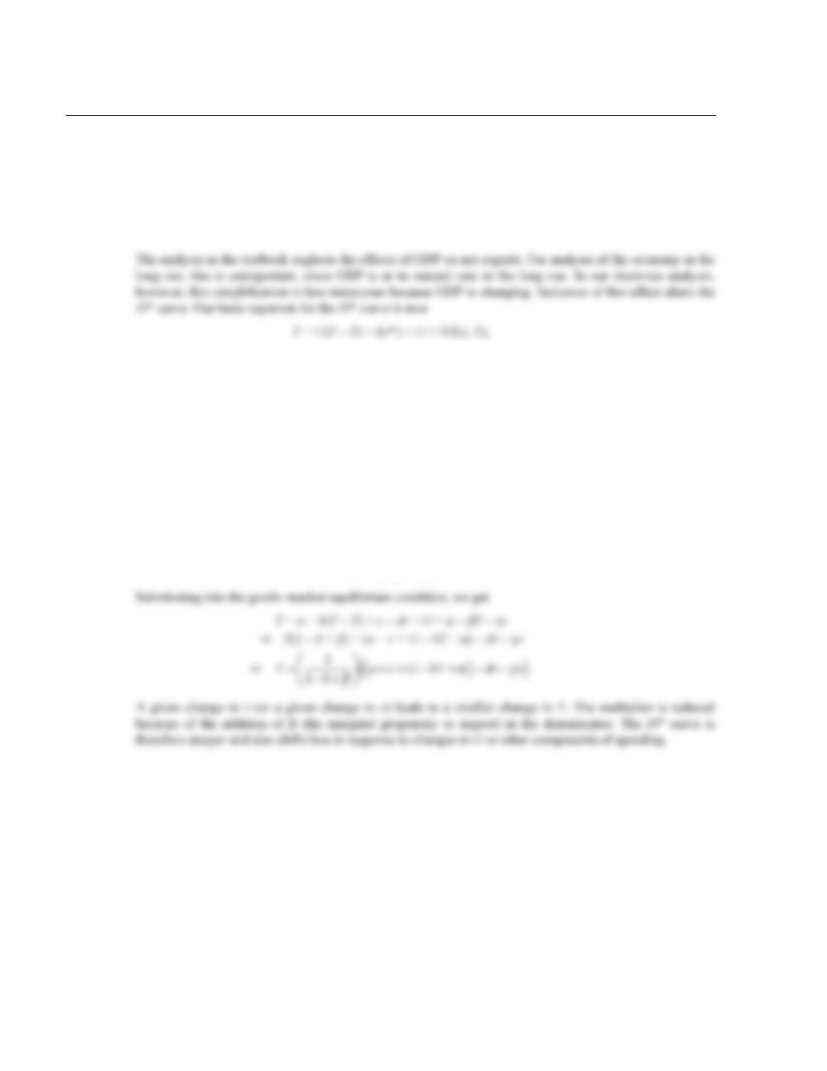
When GDP increases, so does consumption. Since consumers spend money on imported as well as
domestic goods, it seems likely that imports also tend to increase when people’s income increases.
Remembering that net exports is the difference between exports and imports, it follows that we should
expect net exports to depend (negatively) on both the exchange rate and the level of GDP:
NX = NX(e, Y).
or, equivalently,
S(Y) – I(r*) = NX(e, Y).
An increase in Y increases saving, implying that the left-hand side of this equation increases. To
maintain equilibrium, the exchange rate must fall, increasing the right–hand side of the equation. This is
why the IS* curve slopes downward. But now there is an extra effect: Higher GDP tends to reduce net
exports and so reduces the right–hand side. This means that the exchange rate must fall farther than was
previously the case to maintain equilibrium in the market for foreign exchange. Increased GDP, in other
words, both decreases the net supply of foreign currency and increases the net demand. Taking account of
the dependence of net exports on GDP implies that the IS* curve is steeper.
We can also see this algebraically. Suppose that
C = a + b(Y – T)
I = c – dr
NX = α – βY – γe.
ADDITIONAL CASE STUDY
13–2 The Rise in the Dollar, 1979–1982
In the early 1980s the United States experienced an unusual combination of tight monetary policy and
1.83 German marks. In 1982 the dollar was worth 248 yen or 2.42 marks. This rise in the value of the
dollar made imported goods less expensive. U.S. firms competing against similar foreign companies, such
296
13–3 Can World Financial Markets Usurp the Power of the Federal
Reserve?
Some commentators in the media have suggested that the Fed has less influence over the U.S. economy
today than it had in the past. Their argument goes roughly as follows:
2. As a result, U.S. interest rates are more determined by developments in world financial markets and
less determined by domestic monetary policy than they were previously.
3. With less control over interest rates, the Fed may soon find itself powerless in the fight against short–
run economic fluctuations.
Does this argument makes sense? Should U.S. policymakers worry that world financial markets will soon
hold the U.S. economy hostage?
The Mundell–Fleming model tells us not to worry. We can interpret statement 1 in the above
argument as claiming that the U.S. economy is becoming less like the closed economy described by the
IS–LM model and more like the small open economy described by the Mundell–Fleming model. Let’s
ADDITIONAL CASE STUDY
13–4 Bretton Woods
Much of the world operated under fixed exchange rates between 1944 and 1971, as established in the
Bretton Woods agreement. An international conference held in Bretton Woods, New Hampshire,
established an international financial system, including the International Monetary Fund (IMF). All
currencies were pegged (within a 1 percent band) to the dollar, implying that the U.S. dollar was the
billion). If foreign central banks had all tried to convert their dollars into gold, the United States could not
have supplied that gold. In August 1971, fearing such a run against the gold reserves, President Nixon
ended the convertibility of dollars into gold, effectively ending the Bretton Woods period (although the
system was not formally abandoned until early 1973).
Allan Meltzer suggests that the Bretton Woods system failed in part because of U.S. policy.3 As
ADDITIONAL CASE STUDY
13–5 Finland in the 1990s
Finland was an economic success story in the 1980s. Real GDP growth was averaging over 3 percent per
year in the mid–1980s and rose to 4.9 percent in 1988 and 5.7 percent in 1989.1 At that time it was
operating under a system of fixed exchange rates.
But disaster struck in the early 1990s. Real GDP growth was zero in 1990 and real GDP fell by 7.1
percent in 1991, 3.6 percent in 1992, and 1.2 percent in 1993. Between 1990 and 1993 output declined by
nearly 12 percent.
What caused this extraordinarily severe recession? One explanation is the collapse of the economies
of the former Soviet Union. Finland is a small open economy, in which exports account for over 20
percent of GDP. Prior to its collapse, the Soviet Union was the destination for about 17 percent of Finnish
exports. But between 1990 and 1991, this component of exports fell by almost 72 percent. In the Mundell–