205
WHAT’S NEW IN THE EIGHTH EDITION:
There are no major changes to this chapter.
LEARNING OBJECTIVES:
By the end of this chapter, students should understand:
➢ what items are included in a firm’s costs of production.
➢ the link between a firm’s production process and its total costs.
➢ the meaning of average total cost and marginal cost and how they are related.
➢ the shape of a typical firm’s cost curves.
➢ the relationship between short-run and long-run costs.
CONTEXT AND PURPOSE:
Chapter 13 is the first chapter in a five-chapter sequence dealing with firm behavior and the organization
of industry. It is important that students become comfortable with the material in Chapter 13 because
Chapters 14 through 17 are based on the concepts developed in Chapter 13. To be more specific,
Chapter 13 develops the cost curves on which firm behavior is based. The remaining chapters in this
section (Chapters 14-17) use these cost curves to develop the behavior of firms in a variety of different
KEY POINTS:
• The goal of firms is to maximize profit, which equals total revenue minus total cost.
THE COSTS OF PRODUCTION
13
206 ❖ Chapter 13/The Costs of Production
• When analyzing a firm’s behavior, it is important to include all the opportunity costs of production.
Some of the opportunity costs, such as the wages a firm pays its workers, are explicit. Other
opportunity costs, such as the wages the firm owner gives up by working at the firm rather than
taking another job, are implicit. Economic profit takes both explicit and implicit costs into account,
whereas accounting profits consider only explicit costs.
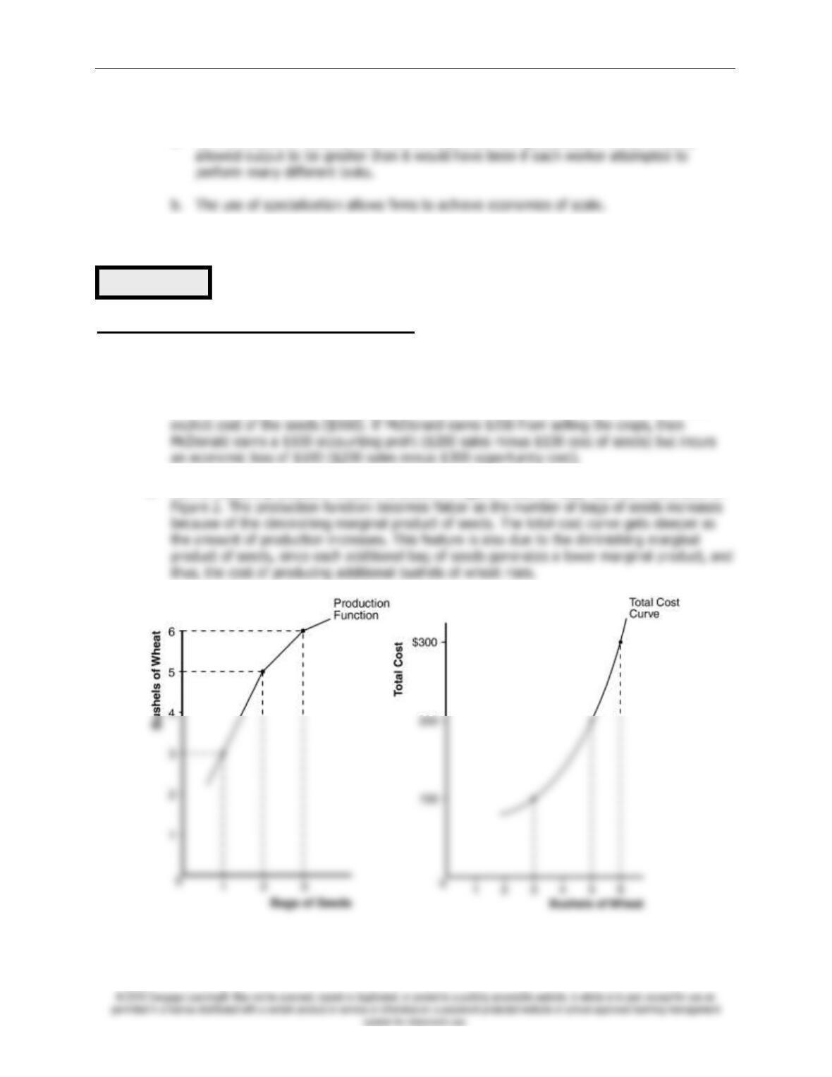
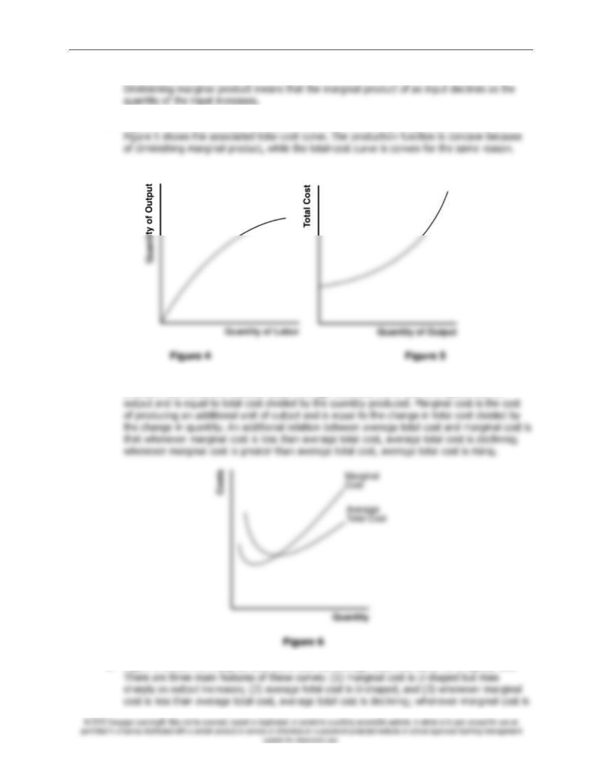
• A firm’s costs reflect its production process. A typical firm’s production function gets flatter as the
quantity of an input increases, displaying the property of diminishing marginal product. As a result, a
firm’s total-cost curve gets steeper as the quantity produced rises.
• From a firm’s total cost, two related measures of cost are derived. Average total cost is total cost
divided by the quantity of output. Marginal cost is the amount by which total cost rises if output
increases by one unit.
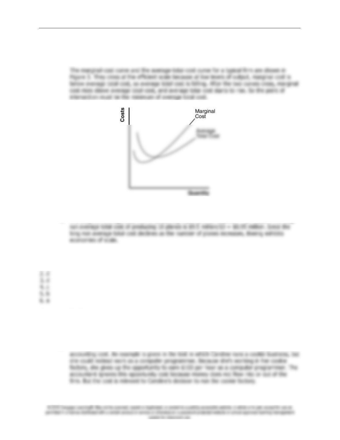
• When analyzing firm behavior, it is often useful to graph average total cost and marginal cost. For a
typical firm, marginal cost rises with the quantity of output. Average total cost first falls as output
increases and then rises as output increases further. The marginal-cost curve always crosses the
average-total-cost curve at the minimum of average total cost.
• A firm’s costs often depend on the time horizon considered. In particular, many costs are fixed in the
short run but variable in the long run. As a result, when the firm changes its level of production,
average total cost may rise more in the short run than in the long run.
CHAPTER OUTLINE:
I. What Are Costs?
A. Total Revenue, Total Cost, and Profit
1. The goal of a firm is to maximize profit.
This is an extremely important chapter, and it is critical that students have an
understanding of the important principles developed here to follow the material
presented in the next several chapters. Do not be surprised at the number of
students who are unfamiliar with such seemingly simple concepts as revenue, costs,
and profits.
Point out to students that it is possible for firm owners to have different goals, but
the one motive that makes the most accurate prediction about how firm managers
behave is the assumption of profit maximization. To help illustrate this sometimes-
Chapter 13/The Costs of Production ❖ 207
2. Definition of total revenue: the amount a firm receives for the sale of its output.
B. Costs as Opportunity Costs
1. Principle #2: The cost of something is what you give up to get it.
2. The costs of producing an item must include all of the opportunity costs of inputs used in
production.
3. Total opportunity costs include both implicit and explicit costs.
c. The total cost of a business is the sum of explicit costs and implicit costs.
d. This is the major way in which accountants and economists differ in analyzing the
performance of a business.
e. Accountants focus on explicit costs, while economists examine both explicit and implicit
costs.
C. The Cost of Capital as an Opportunity Cost
1. The opportunity cost of financial capital is an important cost to include in any analysis of firm
performance.
2. Example: Caroline uses $300,000 of her savings to start her firm. It was in a savings account
paying 5% interest.
Total Revenue = Price Quantity
Students rarely have trouble understanding the concept of explicit costs. However,
they do often have difficulty understanding the nature of implicit costs. Make sure
that they grasp the concept here, because it is important in understanding why firms
continue to operate even if they are earning zero economic profit in the long run.
208 ❖ Chapter 13/The Costs of Production
D. Economic Profit versus Accounting Profit
1. Figure 1 highlights the differences in the ways in which economists and accountants calculate
profit.
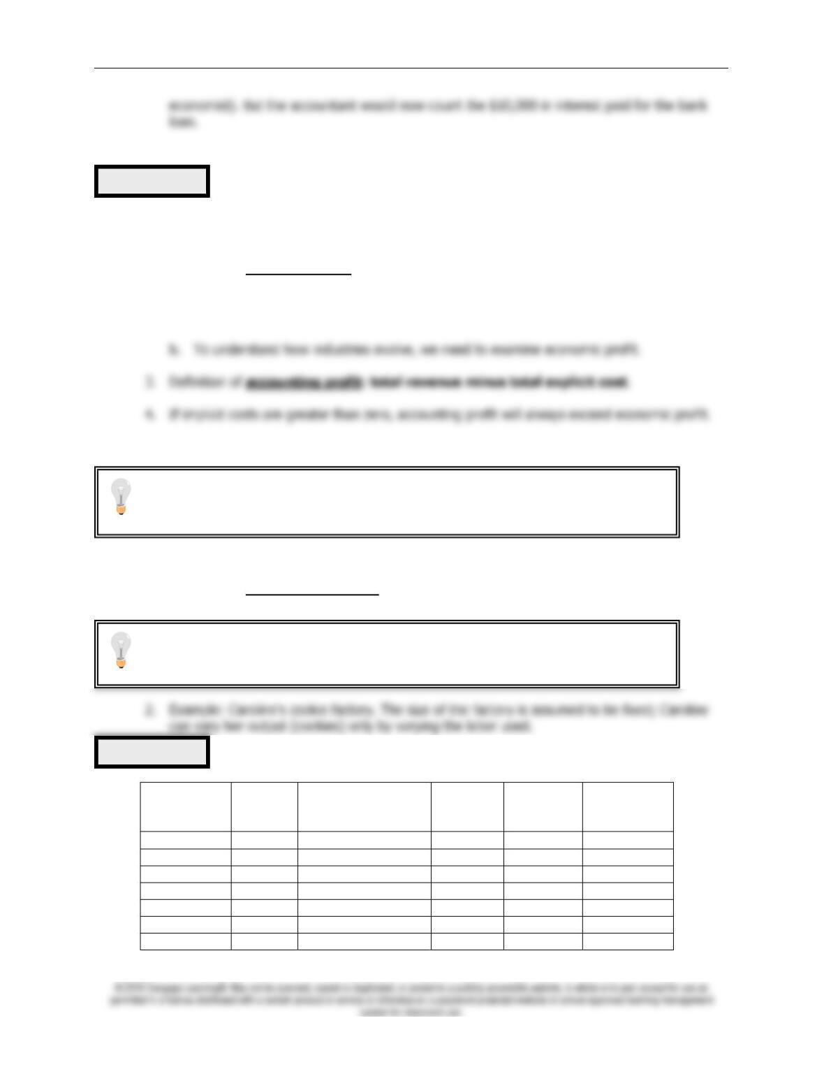
2. Definition of economic profit: total revenue minus total cost, including both explicit
and implicit costs.
a. Economic profit is what motivates firms to supply goods and services.
II. Production and Costs
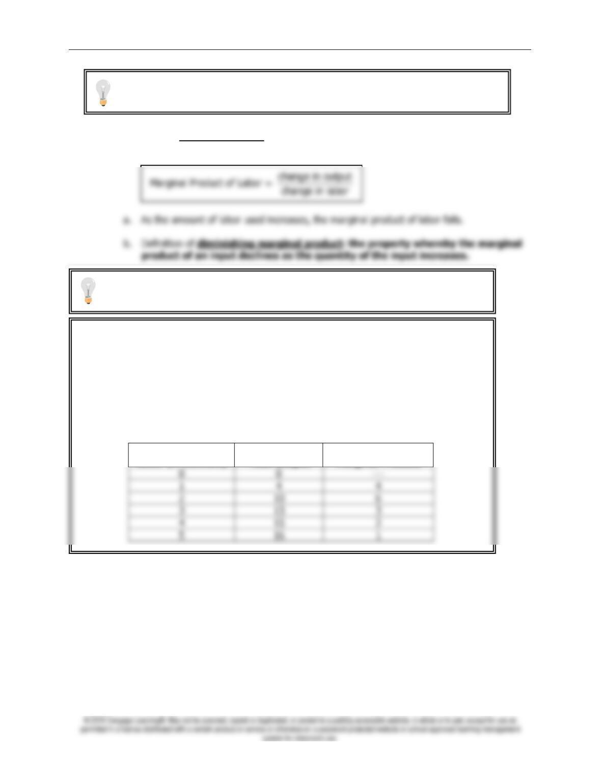
A. The Production Function
1. Definition of production function: the relationship between quantity of inputs used
to make a good and the quantity of output of that good.
(1)
Number of
Workers
(2)
Output
(3)
Marginal Product
of Labor
(4)
Cost of
Factory
(5)
Cost of
Workers
(6)
Total Cost
of Inputs
0
0
—
$30
$0
$30
1
50
50
30
10
40
2
90
40
30
20
50
3
120
30
30
30
60
4
140
20
30
40
70
5
150
10
30
50
80
6
155
5
30
60
90
Figure 1
Table 1
You may want to give students a handout that summarizes the definitions and
provides them an opportunity to practice the calculations in this chapter. (See the
alternative classroom examples.)
It will be beneficial at this point to distinguish between the long run and the short
run. This will help students understand the distinction between fixed inputs and
variable inputs.
Chapter 13/The Costs of Production ❖ 209
3. Definition of marginal product: the increase in output that arises from an additional
unit of input.
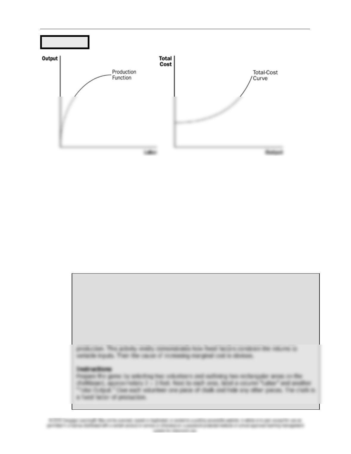
4. We can draw a graph of the firm’s production function by plotting the level of labor (
x
-axis)
against the level of output (
y
-axis).
Go through this table, column by column. Make sure that students understand the
calculations involved.
Point out that diminishing marginal returns is a result of fixed inputs and, therefore is
a short-run phenomenon.
ALTERNATIVE CLASSROOM EXAMPLE:
Consider the short-run production of a small firm that makes sweaters. These sweaters are
made using a combination of labor and knitting machines. In the short run, the firm has
signed a lease to rent one machine. Therefore, in the short run, the firm cannot vary the
amount of knitting machines it uses. However, the firm can vary the amount of labor it
employs.
Columns (1) and (2) in the table below show the production level that the firm can
achieve at various amounts of labor:
(1)
Labor (# workers)
(2)
Total Output
(3)
Marginal Product
210 ❖ Chapter 13/The Costs of Production
a. The slope of the production function measures marginal product.
b. Diminishing marginal product can be seen from the fact that the slope falls as the
amount of labor used increases.
B. From the Production Function to the Total-Cost Curve
1. We can draw a graph of the firm’s total cost curve by plotting the level of output (
x
-axis)
against the total cost of producing that output (
y
-axis).
a. The total cost curve gets steeper and steeper as output rises.
b. This increase in the slope of the total cost curve is also due to diminishing marginal
product: As Caroline increases the production of cookies, her kitchen becomes
overcrowded, and she needs a lot more labor.
Activity 1—Growing Rice on a Chalkboard
Type: In-class demonstration
Topics: Diminishing returns and increasing costs
Materials needed: Chalkboard and chalk
Time: 25 minutes
Class limitations: Works in classes with more than 15 students
Purpose
Students often have difficulty understanding why diminishing returns exist in short-run
Figure 2
Chapter 13/The Costs of Production ❖ 211
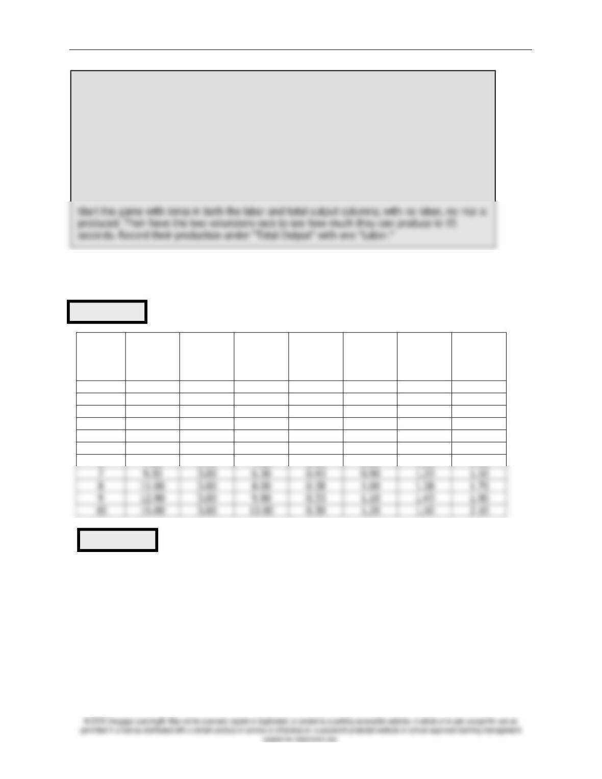
III. The Various Measures of Cost
A. Example: Conrad’s Coffee Shop
(1)
Output
(2)
Total
Cost
(3)
Fixed
Cost
(4)
Variable
Cost
(5)
Average
Fixed
Cost
(6)
Average
Variable
Cost
(7)
Average
Total
Cost
(8)
Marginal
Cost
0
$3.00
$3.00
$0
—
—
—
—
1
3.30
3.00
0.30
$3.00
$0.30
$3.30
$0.30
2
3.80
3.00
0.80
1.50
0.40
1.90
0.50
3
4.50
3.00
1.50
1.00
0.50
1.50
0.70
4
5.40
3.00
2.40
0.75
0.60
1.35
0.90
5
6.50
3.00
3.50
0.60
0.70
1.30
1.10
6
7.80
3.00
4.80
0.50
0.80
1.30
1.30
7
9.30
3.00
6.30
0.43
0.90
1.33
1.50
8
11.00
3.00
8.00
0.38
1.00
1.38
1.70
9
12.90
3.00
9.90
0.33
1.10
1.43
1.90
15.00
3.00
12.00
0.30
1.20
1.50
2.10
The volunteers are farmers and the outlined areas are their farm fields. They produce rice by
writing the word “RICE” in large letters inside their own field. The letters need to be at least
three inches high. They want to produce as much rice as possible in each 15-second time
period.
The variable input in this example is labor. The game is played repeatedly, adding another
student each period. Eventually five students will be crowded around each “field” trying to
write with a tiny piece of chalk.
The constraints from the fixed factors are physically demonstrated.
Table 2
Figure 3
212 ❖ Chapter 13/The Costs of Production
B. Fixed and Variable Costs
1. Definition of fixed costs: costs that do not vary with the quantity of output
produced.
2. Definition of variable costs: costs that do vary with the quantity of output
produced.
3. Total cost is equal to fixed cost plus variable cost.
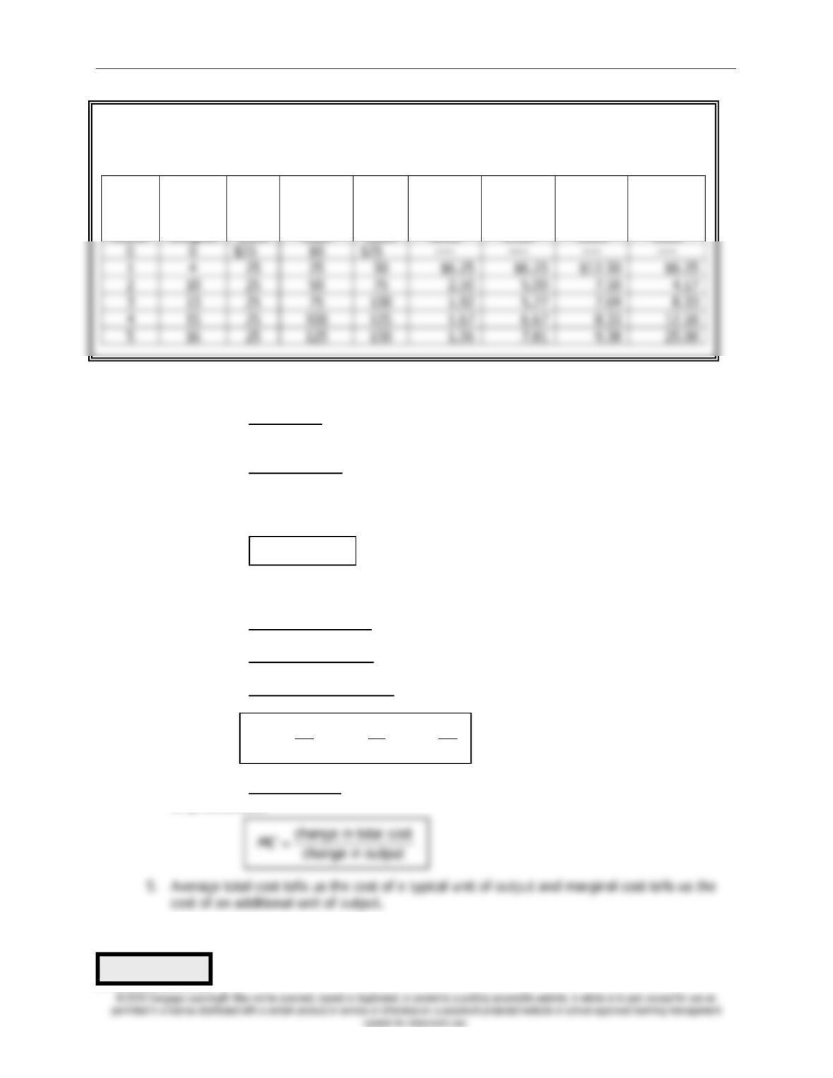
C. Average and Marginal Cost
1. Definition of average total cost: total cost divided by the quantity of output.
2. Definition of average fixed cost: fixed costs divided by the quantity of output.
3. Definition of average variable cost: variable costs divided by the quantity of output.
4. Definition of marginal cost: the increase in total cost that arises from an extra unit
of production.
D. Cost Curves and Their Shapes
;;
TC VC FC
ATC AVC AFC
Q Q Q
= = =
Figure 4
TC FC VC
=+
ALTERNATIVE CLASSROOM EXAMPLE:
Consider the sweater manufacturer (described earlier). The firm is currently renting one machine
for $25 per day. Each worker is also paid $25 per day.
(1)
Labor
(2)
Output
(3)
Fixed
Cost
(4)
Variable
Cost
(5)
Total
Cost
(6)
Average
Fixed
Cost
(7)
Average
Variable
Cost
(8)
Average
Total
Cost
(9)
Marginal
Cost
Chapter 13/The Costs of Production ❖ 213
1. Rising Marginal Cost
a. This occurs because of diminishing marginal product.
2. U-Shaped Average Total Cost
a. Average total cost is the sum of average fixed cost and average variable cost.
b.
AFC
declines as output expands and
AVC
typically increases as output expands.
AFC
is
high when output levels are low. As output expands,
AFC
declines pulling
ATC
down. As
fixed costs get spread over a large number of units, the effect of
AFC
on
ATC
falls and
ATC
begins to rise because of diminishing marginal product.
c. Definition of efficient scale: the quantity of output that minimizes average total
cost.
3. The Relationship between Marginal Cost and Average Total Cost
ATC AFC AVC
=+
214 ❖ Chapter 13/The Costs of Production
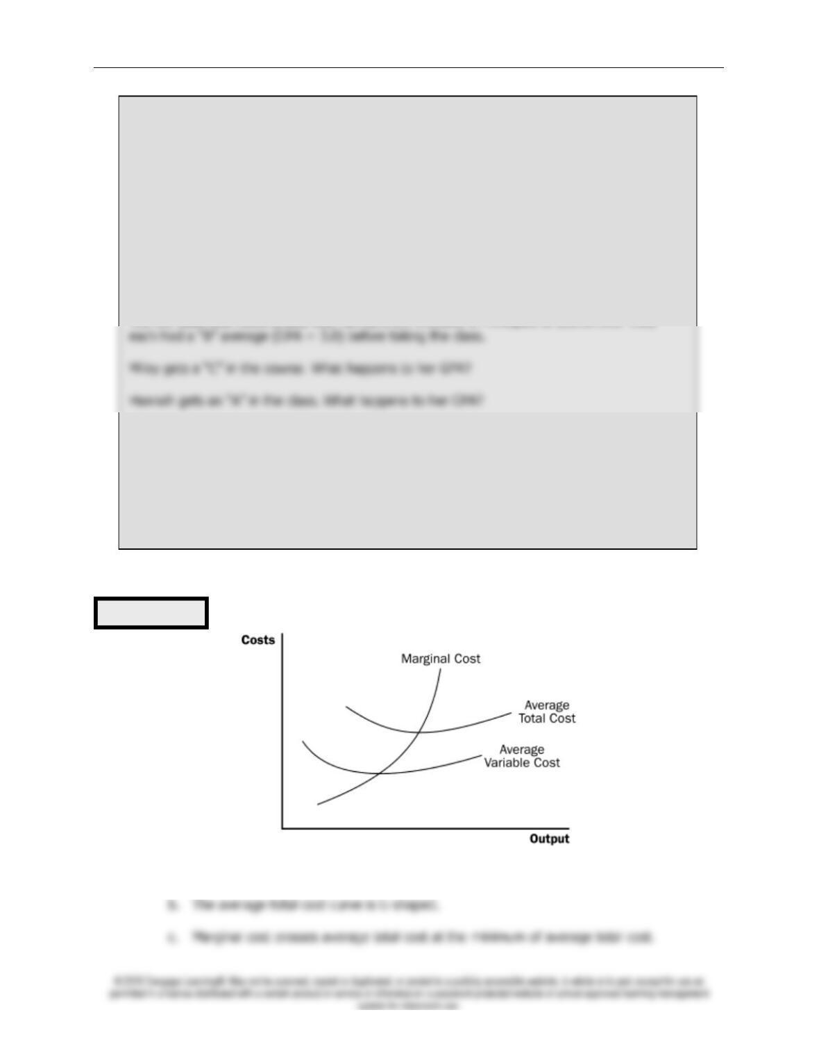
4. Typical Cost Curves
a. Marginal cost eventually rises with output.
Activity 2—Average and Marginal Grades
Type: In-class demonstration
Topics: Relationship between marginal and average cost
Materials needed: None
Time: 5 minutes
Class limitations: Works in any size class
Purpose
This quick exercise uses an analogy to illustrate to students that they already know the
relation between marginal values and averages.
Instructions
Tell the class that twins (Miley and Hannah) are enrolled in Principles of Economics. They
Common Answers and Points for Discussion
Students will likely know that Miley will have a lower GPA and Hannah a higher GPA. A
“marginal” grade lower than the average will pull down the average. A “marginal” grade
higher than the average will increase the average.
The same is true of marginal cost and average costs. If marginal cost is less than average
cost, average cost will fall. If marginal cost is higher than average cost, average cost will rise.
Figure 5
Chapter 13/The Costs of Production ❖ 215
IV. Costs in the Short Run and in the Long Run
A. The division of total costs into fixed and variable costs will vary from firm to firm.
B. Some costs are fixed in the short run, but all are variable in the long run.
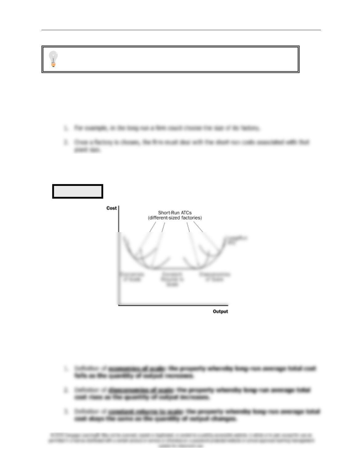
C. The long-run average-total-cost curve lies along the lowest points of the short-run average-total-
cost curves because the firm has more flexibility in the long run to deal with changes in
production.
D. The long-run average-total-cost curve is typically U-shaped, but is much flatter than a typical
short-run average-total-cost curve.
E. The length of time for a firm to get to the long run will depend on the firm involved.
F. Economies and Diseconomies of Scale
Figure 6
Emphasize that these cost curves include ALL costs for the resources needed to
produce the good. Thus, both explicit costs and implicit costs are included.
216 ❖ Chapter 13/The Costs of Production
4.
FYI: Lessons from a Pin Factory
a. In
The Wealth of Nations,
Adam Smith described how specialization in a pin factory
V. Table 3 provides a summary of all of the various cost definitions used throughout this chapter.
SOLUTIONS TO TEXT PROBLEMS:
Quick Quizzes
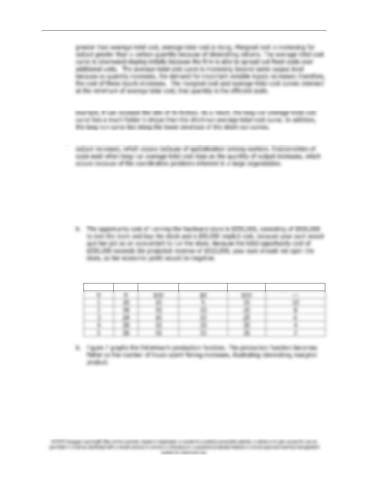
1. Farmer McDonald’s opportunity cost is $300, consisting of 10 hours of lessons at $20 an hour
that he could have been earning plus $100 in seeds. His accountant would only count the
2. Farmer Jones’s production function is shown in Figure 1 and her total-cost curve is shown in
Figure 1 Figure 2
Table 3
Chapter 13/The Costs of Production ❖ 217
3. The average total cost of producing 5 cars is $250,000/5 = $50,000. Since total cost rose
from $225,000 to $250,000 when output increased from 4 to 5, the marginal cost of the fifth
car is $25,000.
Figure 3
4. The long-run average total cost of producing 9 planes is $9 million/9 = $1 million. The long-
Chapter Quick Quiz
1. a
Questions for Review
1. The relationship between a firm’s total revenue, profit, and total cost is profit equals total
revenue minus total costs.
2. An accountant would not count the owner’s opportunity cost of alternative employment as an
218 ❖ Chapter 13/The Costs of Production
3. Marginal product is the increase in output that arises from an additional unit of input.
4. Figure 4 shows a production function that exhibits diminishing marginal product of labor.
5. Total cost consists of the costs of all inputs needed to produce a given quantity of output. It
includes fixed costs and variable costs. Average total cost is the cost of a typical unit of
6. Figure 6 shows the marginal-cost curve and the average-total-cost curve for a typical firm.
Chapter 13/The Costs of Production ❖ 219
7. In the long run, a firm can adjust the factors of production that are fixed in the short run; for
8. Economies of scale exist when long-run average total cost decreases as the quantity of
Problems and Applications
1. a. opportunity cost; b. average total cost; c. fixed cost; d. variable cost; e. total cost; f.
marginal cost.
2. a. The opportunity cost of something is what must be given up to acquire it.
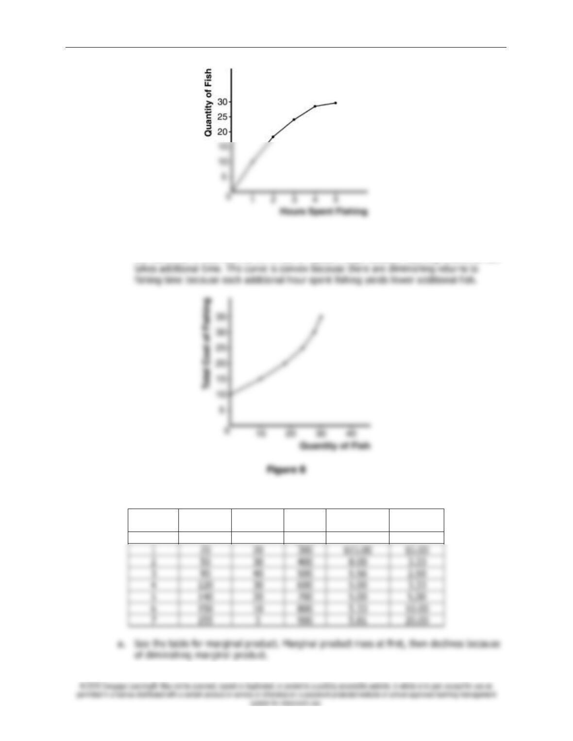
3. a. The following table shows the marginal product of each hour spent fishing:
Hours
Fish
Fixed Cost
Variable Cost
Total Cost
Marginal Product
220 ❖ Chapter 13/The Costs of Production
Figure 7
c. The table shows the fixed cost, variable cost, and total cost of fishing. Figure 8 shows
the fisherman’s total-cost curve. It has an upward slope because catching additional fish
4. Here is the completed table:
Workers
Output
Marginal
Product
Total
Cost
Average
Total Cost
Marginal
Cost
0
0
—
$200
—
—
1
2
8.00
3
5.56
4
5.00
5
5.00
6
5.33
7
5.81
Chapter 13/The Costs of Production ❖ 221
b. See the table for total cost.
5. At an output level of 600 players, total cost is $180,000 (600 × $300). The total cost of
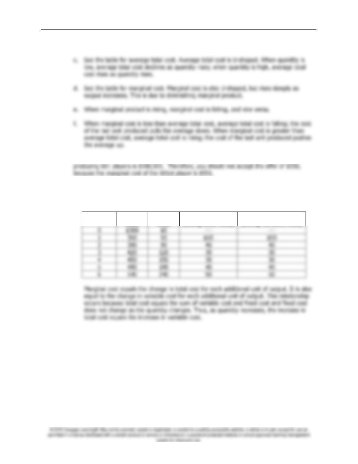
6. a. The fixed cost is $300, because fixed cost equals total cost minus variable cost. At an
output of zero, the only costs are fixed cost.
b.
Quantity
Total
Cost
Variable
Cost
Marginal Cost
(using total cost)
Marginal Cost
(using variable cost)
7. The following table illustrates average fixed cost (
AFC
), average variable cost (
AVC
), and
average total cost (
ATC
) for each quantity. The efficient scale is 4 houses per month,
because that minimizes average total cost.
222 ❖ Chapter 13/The Costs of Production
Quantity
Variable
Fixed
Total
Average
Average
Average
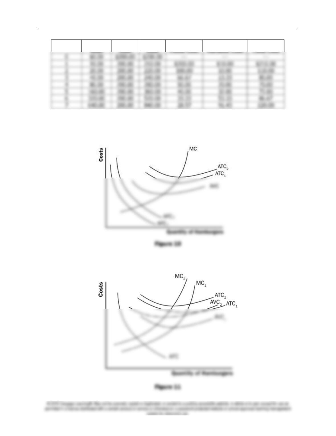
8. a. The lump-sum tax causes an increase in fixed cost. Therefore, as Figure 10 shows, only
average fixed cost and average total cost will be affected.
b. Refer to Figure 11. Average variable cost, average total cost, and marginal cost will all be
greater. Average fixed cost will be unaffected.
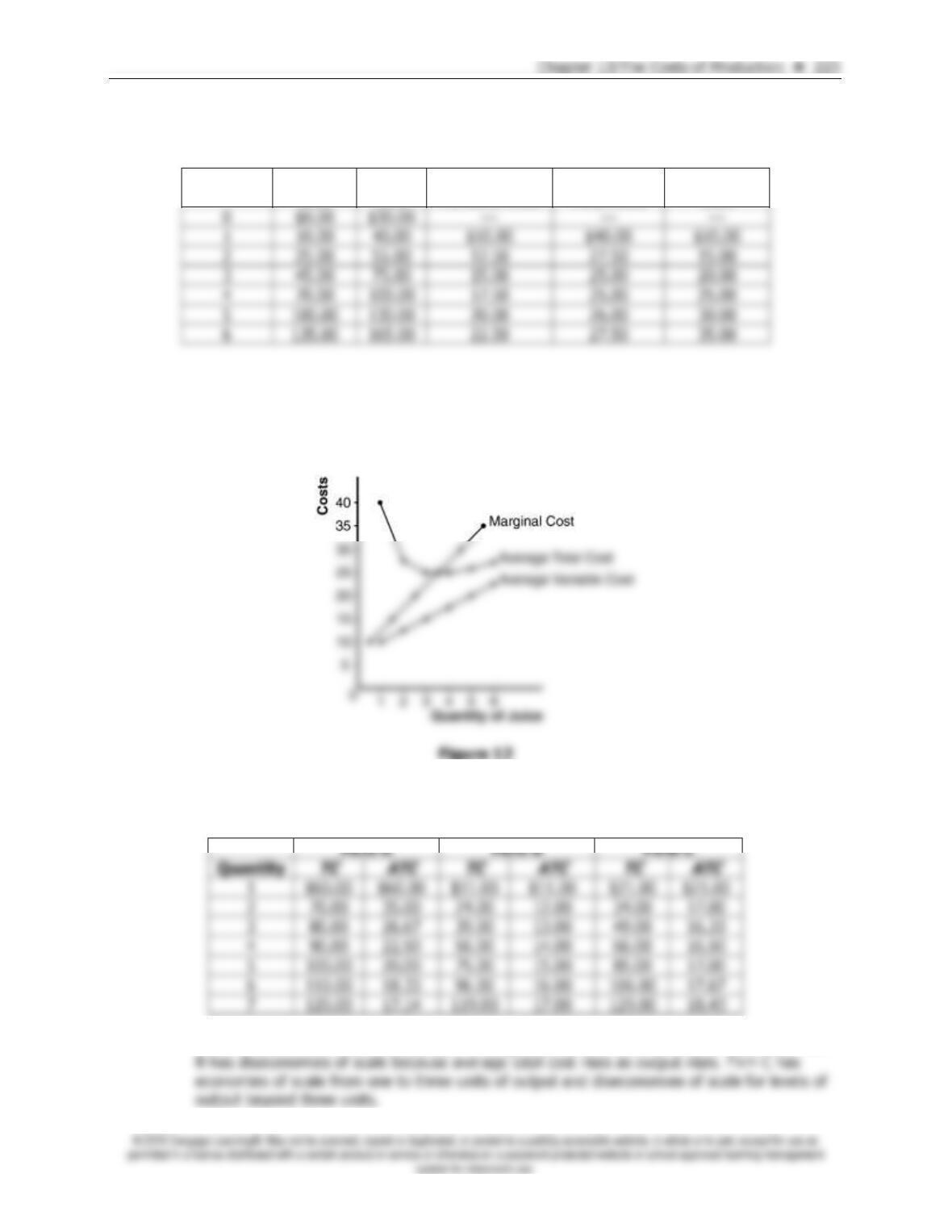
9. a. The following table shows average variable cost (
AVC
), average total cost (
ATC
), and
marginal cost (
MC
) for each quantity.
Quantity
Variable
Cost
Total
Cost
Average
Variable Cost
Average
Total Cost
Marginal
Cost
b. Figure 12 shows the three curves. The marginal-cost curve is below the average-total–
cost curve when output is less than four and average total cost is declining. The
marginal-cost curve is above the average-total-cost curve when output is above four and
average total cost is rising. The marginal-cost curve lies above the average-variable-cost
curve.
Figure 12
10. The following table shows quantity (
Q
), total cost (
TC
), and average total cost (
ATC
) for the
three firms:
Firm A has economies of scale because average total cost declines as output increases. Firm