13 Chapter model 12/12/2018
BUSINESS RISK AND FINANCIAL RISK (Section 13-2)
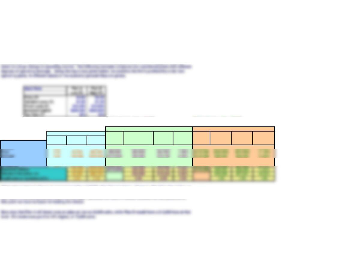
OPERATING LEVERAGE
A‘s break-even units = 50,000. B’s break-even units = 70,000.
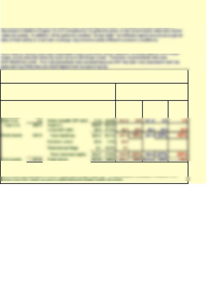
Operating Performance
Units Dollar Operating Operating
Demand Probability Sold Sales Costs EBIT EBIT(1 – T) ROIC Costs EBIT EBIT (1 – T) ROIC
Good 0.20 160,000 $320,000 $265,000 $55,000 $41,250 20.63% $230,000 $90,000 $67,500 33.75%
Which plan is better? Based on expected profits and ROIC, Plan B looks better. However, Plan B is also riskier, as
measured by the standard deviation (s) and the coefficient of variation (CV). So, we face a tradeoff between risk
and return–B is more profitable, but A is less risky. Someone will have to choose between the two plans, but at
Plan B: High Fixed, Low Variable Costs
In this chapter, we introduce two new dimensions of risk, business risk and financial risk. Business risk is the risk
inherent in the firm’s operations, and it would be there even if the firm used no debt. Financial risk is the
additional risk borne by the stockholders as a result of the use of debt.
Operating leverage reflects the degree to which fixed costs are embedded in a firm’s operations. Thus, if a high
percentage of a firm’s costs are fixed, then the firm is said to have high operating leverage because these costs are
incurred even if sales decline. High operating leverage produces a situation where a small change in sales can
Data Applicable to Both Plans
Chapter 13. Capital Structure and Leverage
Plan A: Low Fixed, High Variable Costs
Further discussion of Operating Leverage (Beyond the scope of Concise FFM, but interesting)
1. The beta of the ith asset can be found using this equation:
bi = r i,m ( si / sm )
3. We could calculate the historical R between some traded assets and the market,
and make an educated guess about R for non-traded assets, like Bigbee’s project.
5. We calculated above the s for A and B as follows:
s(A) = 9.26%
s(B) = 18.52%
These betas could be used in the Hamada equation as described
below to bring in financial risk and thus to get an idea of total risk with
different operating and financial plans.
QBE = F / (P − V)
Plan A
QBE, A = F / (P −V)
FINANCIAL RISK
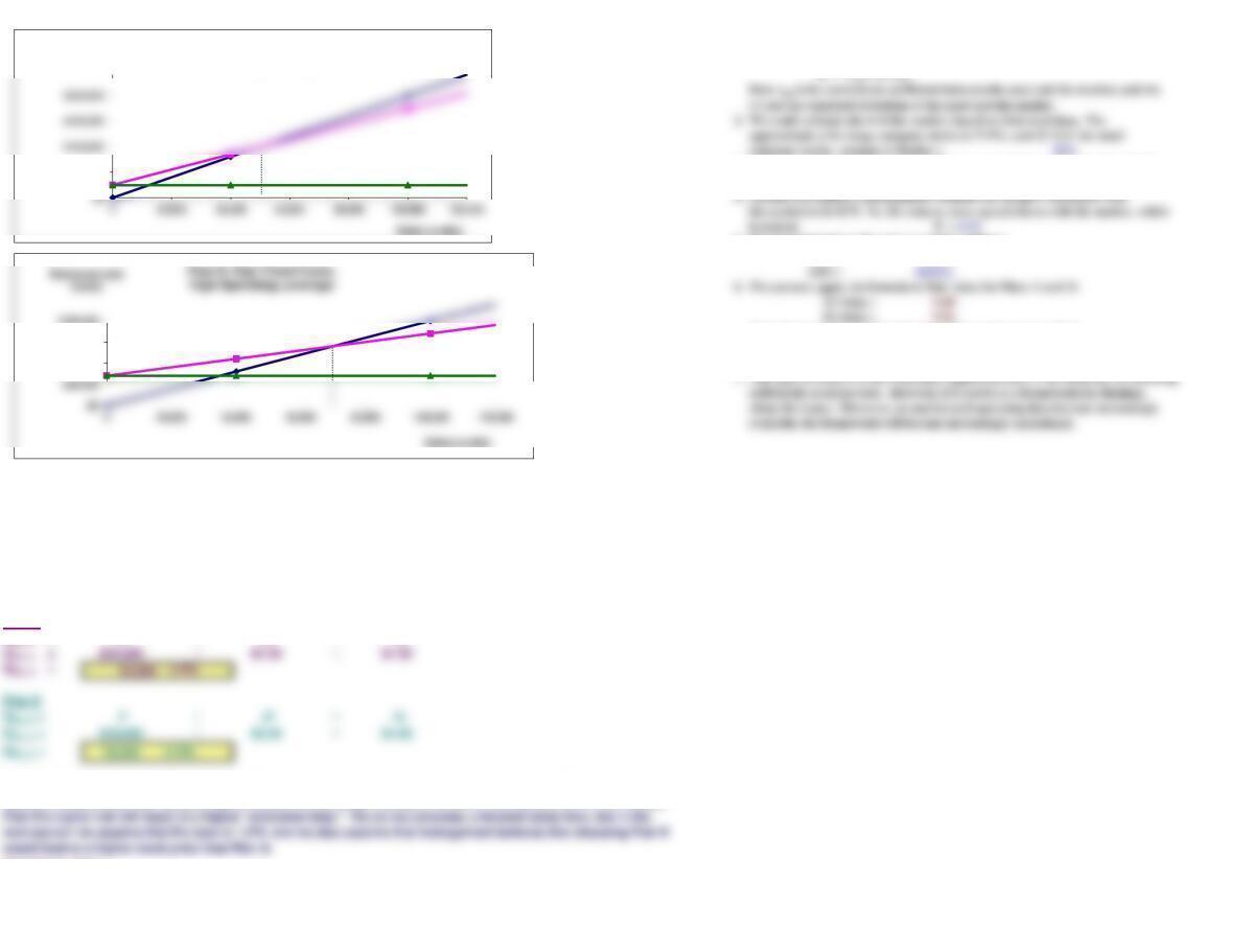
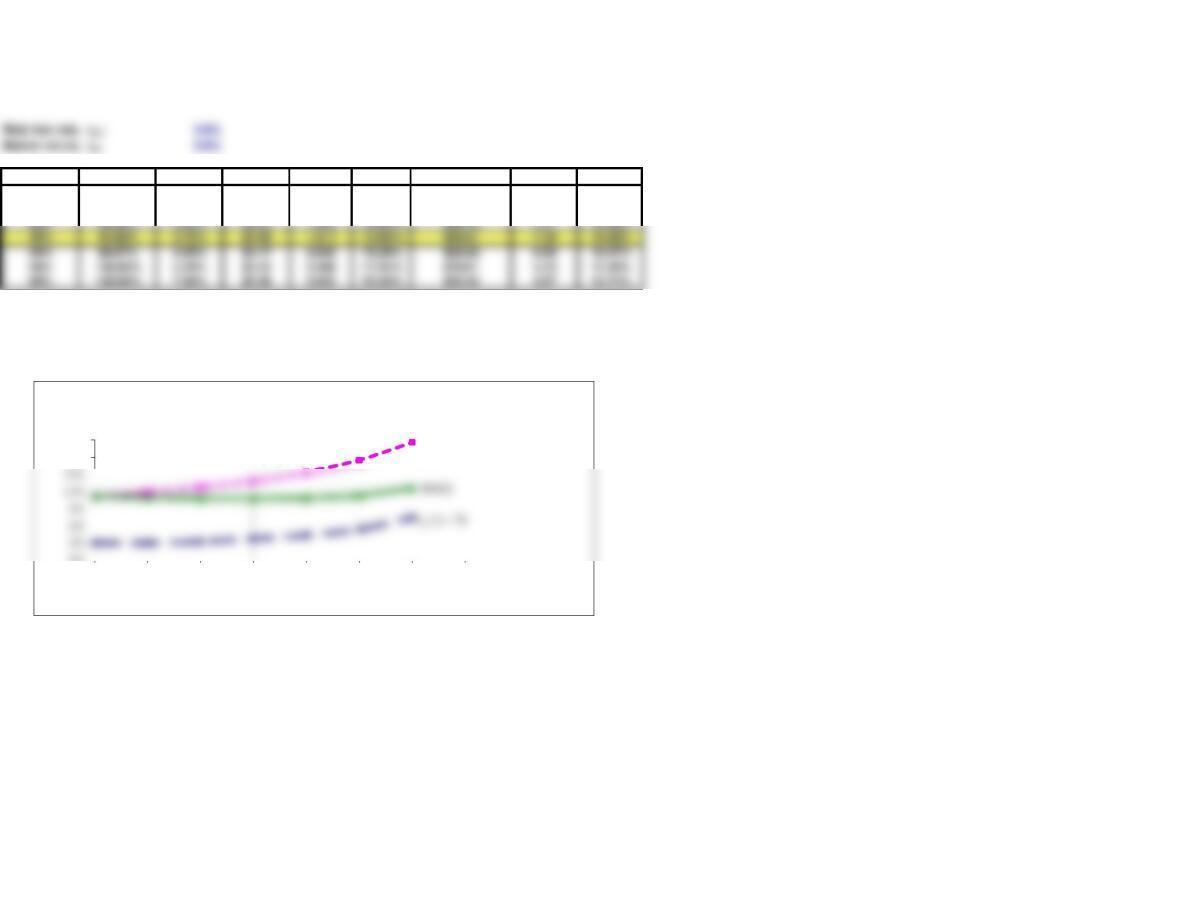
The results generated in the table above are graphed here:
(1) B has a much higher break-even point, and (2) B has more operating leverage in the sense that a given change
in sales leads to a larger change in profits than for A.
We can see from the graph that A‘s break-even point is between 40,000 and 60,000 units and that B’s break-even
point is between 60,000 and 80,000 units, but we cannot tell the exact points. However, we can use the following
formula to find the exact break-even point for both plans:
At this point, we know that Plan B has a higher expected rate of return, but it is also more risky. Our analysis is
based on stand-alone risk. However, given a positive correlation between the firm’s returns and that on the market,
$100,000
$150,000
$200,000
$50,000
Revenues and
Costs
Plan A: Low Fixed Costs,
Low Operating Leverage
2. We could estimate the s of the market, based on historical data. The
approximate s for large company stocks is 27.9%, and 25.76% for small
company stocks. Assume s Market = 25%
Amount Cost of
Borrowed Debt
0% $0 4.0%
10% $20,000 4.0%
The risk of the stock is reflected in the stock’s beta coefficient, and, as we discuss below, beta rises with the use of
debt–the more debt, the higher the beta. The lowest beta is the one that would exist if no debt were used–this is
the “unlevered beta,” and it reflects the firm’s business risk.
Discussions with its bankers indicate that Bigbee can borrow different amounts, but the more it borrows, the
higher the cost of its debt as shown in the table below:
Debt/Capital
Ratio
Financial leverage refers to the use of fixed-income securities (preferred stock and debt) in the capital structure.
The firm has a certain amount of business risk as discussed above in connection with operating leverage. This
business risk is measured by the firm’s “unlevered beta,” which is the beta it would have if it had no debt. If the
Debt Cost Schedule
20% $40,000 4.3%
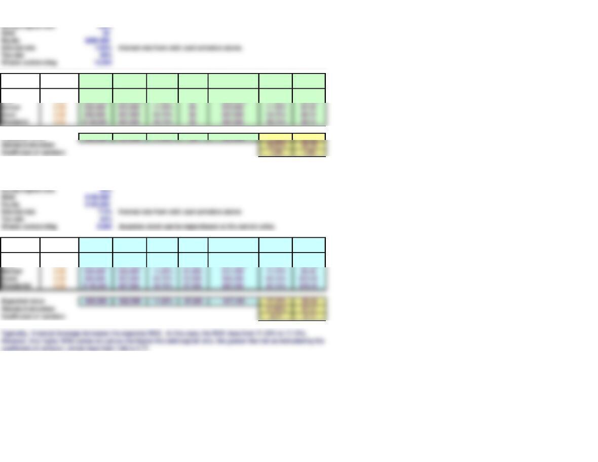
OPTION 1: Finance Plan B entirely with common equity (Equity = 100%, Debt = 0%)
Invested capital $200,000
Debt/Capital ratio 0%
Demand for Net Income =
Product Probability EBIT EBIT(1 − T) ROIC Interest (EBIT − Int)(1 − T) ROE EPS
Terrible
0.05 ($70,000) ($52,500) -26.25% $0 ($52,500) -26.25% ($5.25)
Poor
0.20 ($30,000) ($22,500) -11.25% $0 ($22,500) -11.25% ($2.25)
Expected value $30,000 $22,500 11.25% $0 $22,500 11.25% $2.25
Standard deviation 18.52% $3.70
Coefficient of variation 1.65 1.65
OPTION 2: Finance Plan B with $100,000 of debt and $100,000 of equity (50% equity, 50% debt)
Invested capital $200,000
Debt/Capital ratio 50%
Equity/Capital ratio 50%
Interest rate 7.2% Interest rate from debt cost schedule above.
Tax rate 25%
Shares outstanding 5,000 Assumes stock can be repurchased at the current price.
Demand for Net Income =
Product Probability EBIT EBIT(1 − T) ROIC Interest (EBIT − Int)(1 − T) ROE EPS
Terrible 0.05 ($70,000) ($52,500) -26.25% $7,200 ($57,900) -57.90% ($11.58)
Poor 0.20 ($30,000) ($22,500) -11.25% $7,200 ($27,900) -27.90% ($5.58)
Expected value $30,000 $22,500 11.25% $7,200 $17,100 17.10% $3.42
Standard deviation 37.05% $7.41
Coefficient of variation 2.17 2.17
Equity/Capital ratio 100%
Interest rate 4.00% Interest rate from debt cost schedule above.
Tax rate 25%
Shares outstanding 10,000
Debt/Capital
Ratio
Exp. EPS SD of EPS CV of EPS
50% $3.42 $7.41 2.17
0% $2.25 $3.70 1.65 Minimum risk
10% $2.43 $4.12 1.69
60% $3.38 $9.26 2.74
DETERMINING THE OPTIMAL CAPITAL STRUCTURE (Section 14-3)
THE HAMADA EQUATION
bU1.375
Tax rate 25%
Debt/Capital D/E
bL
0.0 0.00 1.375
0.3 0.43 1.817
0.4 0.67 2.063
0.6 1.50 2.922
Hamada developed his equation by merging the CAPM with the Modigliani-Miller model. We use the model to
determine beta at different amounts of financial leverage, and then use the betas associated with different
debt/capital ratios to find the cost of equity associated with each of those debt/capital ratios. Here is the Hamada
equation:
In the table below, we apply the Hamada equation to Bigbee Electronics, given its unlevered beta and tax rate.
The optimal capital structure is the one that maximizes the stock price, and this is the same one that minimizes the
WACC. To find–or, really, estimate–the optimal capital structure, we need information on how capital structure
In the tables just above, we calculated the expected EPS and risk measures at zero debt and at 50% debt. We can
use an Excel Data Table to calculate these values at a number of different debt/capital ratios, as shown below.
There’s a conflict between risk and return so we must decide what the appropriate tradeoff is, i.e., we must decide
the optimal capital structure.
20% $2.65 $4.63 1.75
Debt/Capital D/E
rd(1 – T) EPS = DPS Est. beta rsEst. Price P/E Ratio WACC
0% 0.00% 3.00% $2.25 1.375 11.25% $20.00 8.89 11.25%
10% 11.11% 3.00% $2.43 1.490 11.94% $20.38 8.38 11.04%
40% 66.67% 4.35% $3.17 2.063 15.38% $20.62 6.50 10.97%
We see that the stock price is maximized, and the WACC is minimized, if the firm finances with 30% debt and 70%
equity. This is the optimal capital structure.
Below, we graph the key data from the table above.
As the table shows, beta rises with financial leverage. With beta specified, we can determine the effects of
leverage on the cost of equity and then on the WACC. Here we assume that the risk-free rate is 3%, the required
return on the market is 9%, and, therefore, the market risk premium is 6%. We also assume that Bigbee pays out all
of its earnings as dividends, hence its earnings and dividends are not expected to grow. Therefore, its stock price
can be found by using the perpetuity equation, Price = Dividend/rs.
0%
18%
21%
0% 10% 20% 30% 40% 50% 60% 70%
Cost of Capital
Debt/Capital Ratio
Effects of Capital Structure on the Cost of Capital
rs
13 Chapter model 12/12/2018
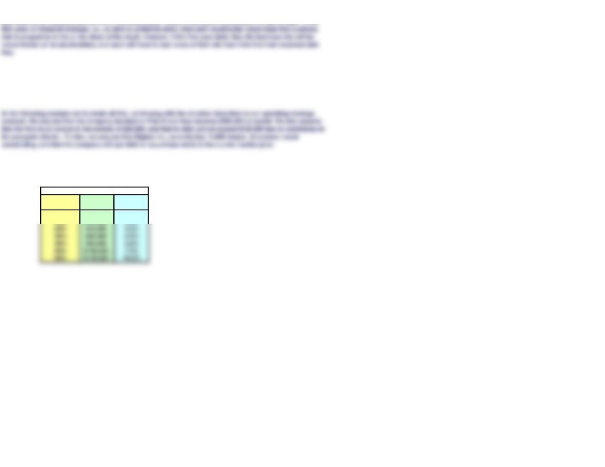
Section 13-1. Book, Market, or Target Weights?
Assets Target %
Cash $8.3 Accounts payable $10.2 13.2% – – – – –
Receivables 16.1 Accruals 5.7 7.4% – – – – –
Inventories 10.0
CAT had 597.63 million shares outstanding, its book value per share was $23.03, and its year-end market price
was $157.58 per share. We do not know its management-determined target capital structure. The 40% debt
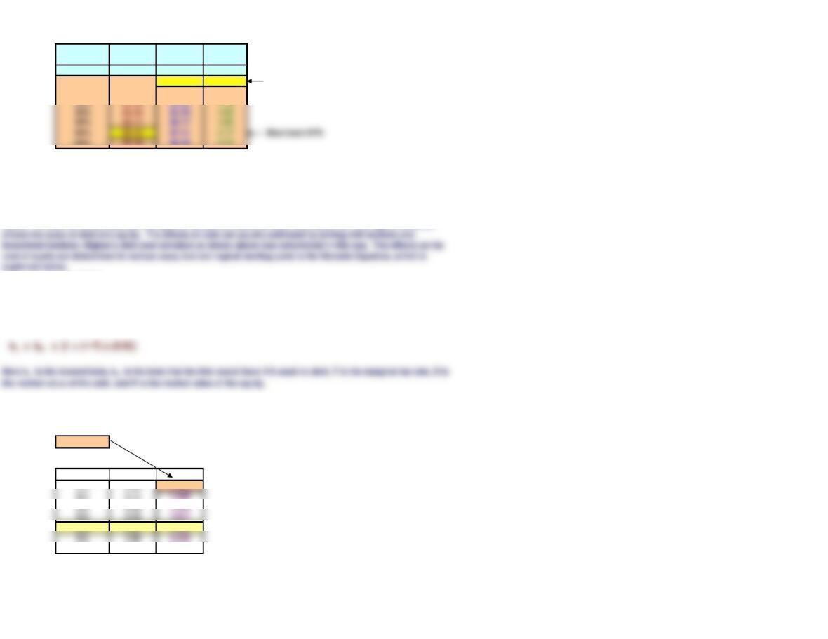
We can think about a firm’s capital structure in three ways: (1) in book value terms, (2) in market value terms,
or (3) as a target capital structure that is not tied directly to either book or market data. The target capital
structure is the one used for the weights when calculating the WACC. The capital structure decision is
We show below, in columns A-H, an abbreviated balance sheet of Caterpillar Inc.(CAT) as of 12/31/17. The
Table 13.1 Caterpillar Inc.’s Book Value, Market Value, and Target Capital Structure
(Dollars in Billions)
Condensed Balance Sheet
Assets and Claims Against Assets At Book Values
Investor supplied capital: Payables and
accruals are excluded because they come
from operations, not from investors
Claims
Book Value
Market Value
2. In CAT‘s case, as is often true, we assume that the market value of the debt is
approximately equal to its book value, but the common stock’s market price differs from
its book value.
3. The stock sells at a price of $157.58 per share versus a book value of $23.03, and the firm
has 597.63 million shares outstanding. Therefore, the market value of the common equity is
4. No distinction is made between common equity raised by issuing stock vs. retaining
earnings when establishing the target capital structure.
5. For illustrative purposes, we assume that CAT has the same cost for long-term bonds and
short-term notes payable, hence it can lump the two together and use a 40% weight for
all investor-supplied debt, i.e., for all debt other than accounts payable and accruals. If
the interest rates varied, then the firm could treat long- and short-term debt separately or
6. If CAT used preferred stock, the market value of that stock would be calculated in the
same way as we calculated the market value of its common equity.
7. Assume that the average interest rate on both short- and long-term new debt is 5%, the
firm’s tax rate is 25%, and its cost of equity is 11%. Here are the WACCs based on book,
market, and target weights:
calculated WACC. The greater the difference between the book and market values of the
stock, and the greater the difference between the costs of debt and equity, the greater
the difference in the calculated WACCs.
8. Generally, a firm’s managers take into account its current and recent past book and
market value structures, as well as those of firms used as benchmarks, when they
like the one we do in the remainder of the chapter.
Accounts payable and accruals come in as a result of operations, not from investors,
so they are not considered to be capital as the term is used here. The capital structure
13 Chapter model 12/12/2018
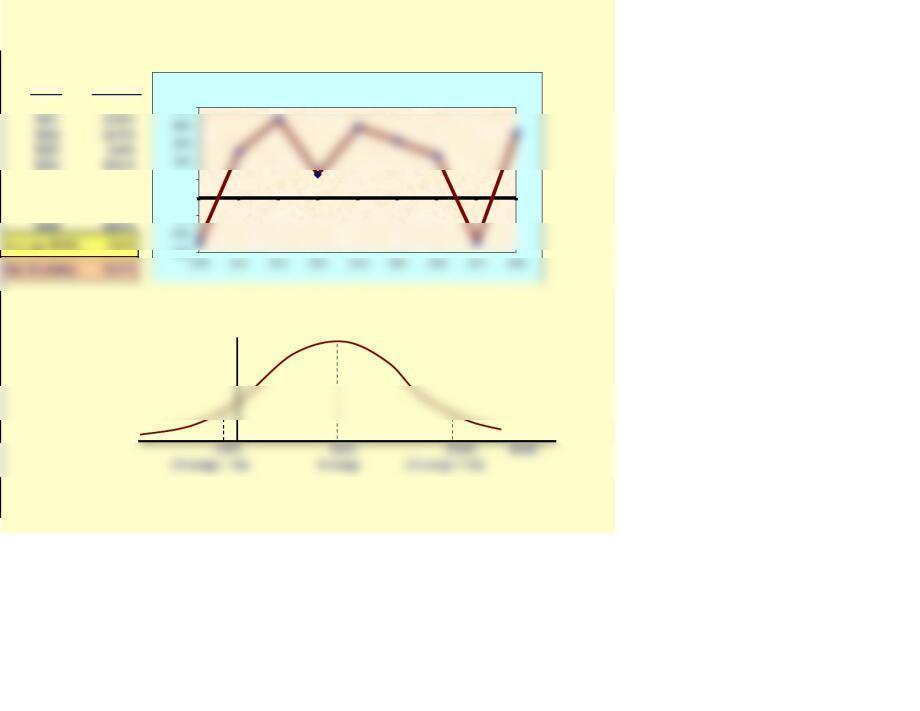
Figure 13.1 Return on Invested Capital (ROIC), 2010−2018
a. ROIC Over Time: An Indicator of Business Risk
Year
ROIC
2010 -12.4%
2015 15.7%
2016 11.5%
2017 -12.2%
b. Probability Distribution of ROIC: Another Indicator of Business Risk
Probability
Since Bigbee has no debt, its ROIC is equal to its ROE, hence we could replace the term
ROIC with ROE. Note, though, that as soon as debt is issued, ROE and ROIC will differ.
-15%
-5%
0%
5%
25%
ROIC
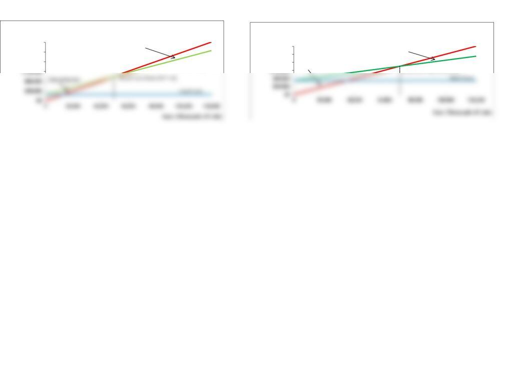
Figure 13.2 Illustration of Operating Leverage 12/12/2018
Plan A Plan B
$160,000
$200,000
$240,000
Revenues and Costs
(Thousands of
Dollars)
Total Operating Costs
Sales Revenues
Operating Profit (EBIT)
$120,000
$160,000
$200,000
$240,000
Revenues and Costs
(Thousands of
Dollars)
Sales Revenues
Total Operating Costs
Break-Even Point (EBIT = 0)
Operating Loss
Operating Profit (EBIT)
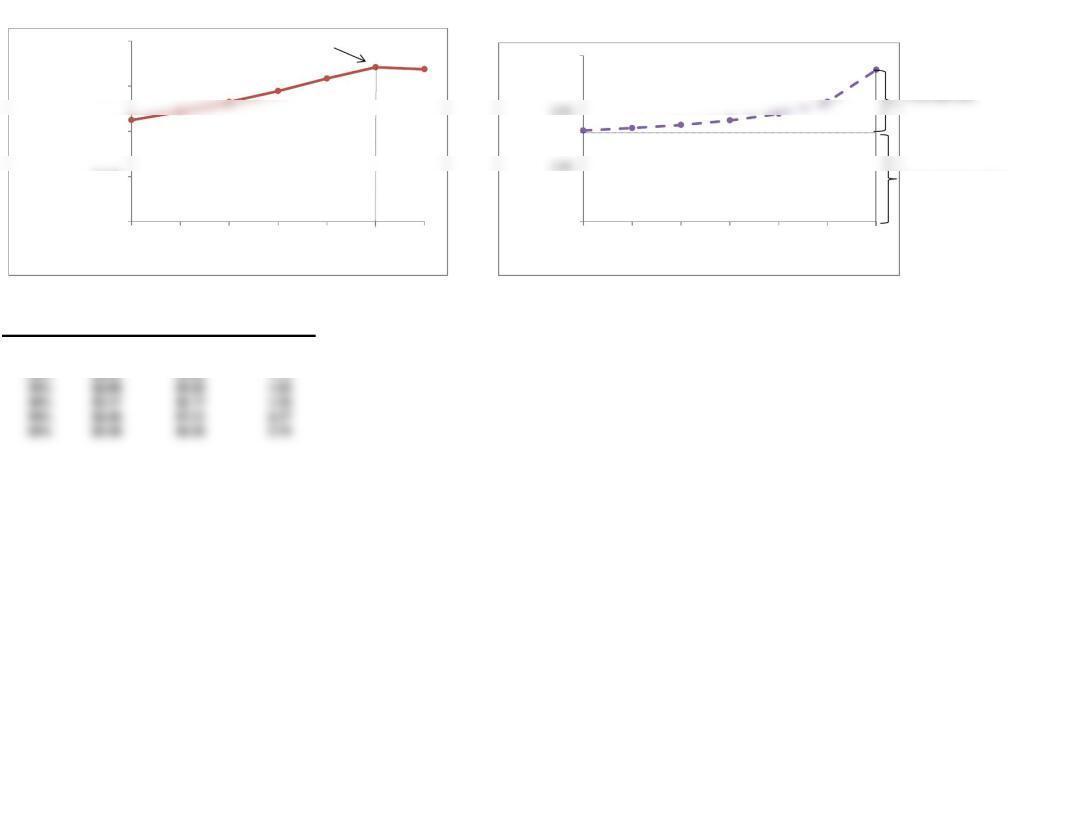
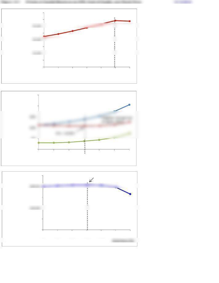
Figure 13.5 Relationships among Expected EPS, Risk, and Financial Leverage
Debt/Capital
Expected
EPS
Standard
Deviation of EPS
Coefficient
of Variation
0% $2.25 $3.70 1.65
10% $2.43 $4.12 1.69
20% $2.65 $4.63 1.75
Basic Business Risk
Additional Risk to Stockholders
from Use of Financial Leverage:
Financial Risk
12/12/2018
$0.00
$1.00
$2.00
$3.00
$4.00
0% 10% 20% 30% 40% 50% 60%
Expected EPS
Debt Ratio (%)
Peak EPS = $3.42
0.00
3.00
0% 10% 20% 30% 40% 50% 60%
Risk
(CVEPS)
Debt Ratio (%)
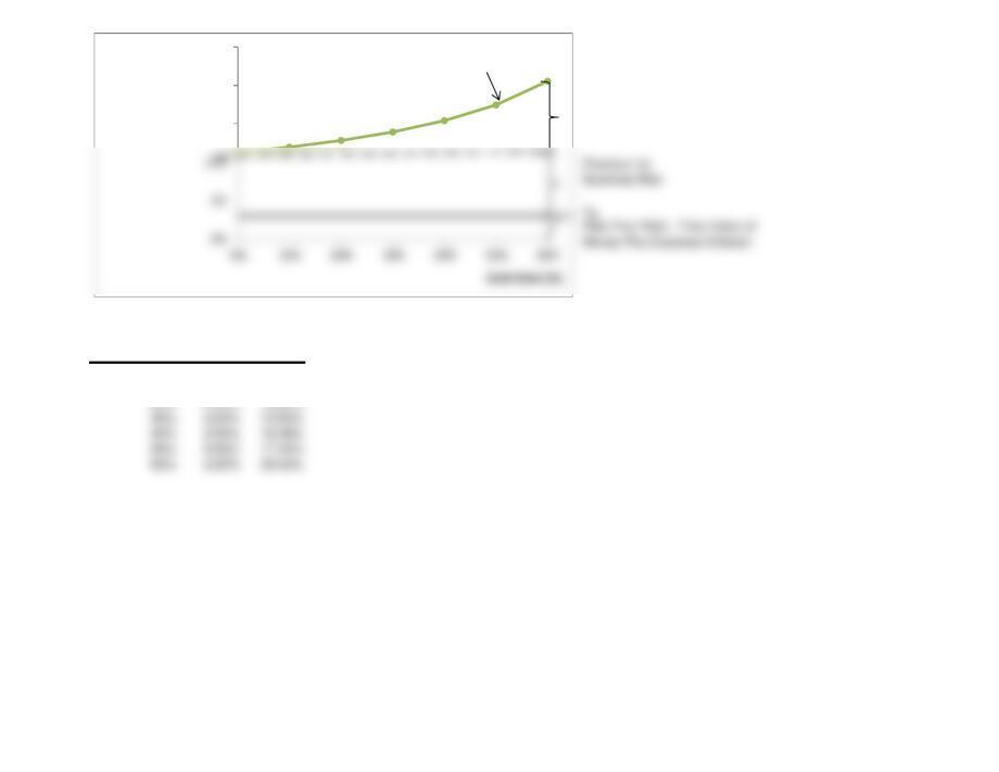
Figure 13.6 Bigbee’s Required Rates of Return on Equity at Different Debt Levels 12/12/2018
Premium for
Financial Risk
Debt/Capital
rRF rs
0% 3.00% 11.25%
10% 3.00% 11.94%
15%
20%
25%
Required Return
on Equity (%)
rS
$0.00
$0.50
$1.50
$2.50
$3.50
$4.00
0% 10% 20% 30% 40% 50% 60%
Expected EPS ($)
Debt Ratio (%)
Maximum EPS = $3.42
0%
5%
20%
25%
0% 10% 20% 30% 40% 50% 60%
Cost of Capital
(%)
Debt Ratio (%)
Cost of Equity, rs
After-Tax Cost of
$0.00
$5.00
$15.00
$25.00
0% 10% 20% 30% 40% 50% 60%
Stock Price ($)
Maximum = $20.81

Debt/Capital D/E
rd(1 – T) EPS = DPS Est. beta rsEst. Price P/E Ratio WACC
0.00% 0.00% 3.00% $2.25 1.375 11.25% $20.00 8.89 11.25%
50.00% 100.00% 5.40% $3.42 2.406 17.44% $19.61 5.73 11.42%
SECTION 13-3 12/12/2018
SOLUTIONS TO SELF-TEST QUESTIONS
bL1.25
Tax rate 25%
bU0.8101
Equity/Capital ratio (Case 1) 1.00
EquityCapital ratio (Case 2) 0.58
4. Use the Hamada equation to calculate the unlevered beta for Firm X with the following data: bL
= 1.25; T = 25%; Debt/Capital = 0.42; Equity/Capital = 0.58.
5a. What would the cost of equity be for Firm X at an Equity/Capital ratio of 1.0 (no debt), assuming
that rRF = 5% and RPM = 4%?
5b. What would the cost of equity be for Firm X at an Equity/Capital ratio of 0.58, assuming that rRF
= 5% and RPM = 4%?
Debt/Capital ratio 0.42
Equity/Capital ratio 0.58