Basic Econometrics, Gujarati and Porter
CHAPTER 13:
ECONOMETRIC MODELING: MODEL SPECIFICATION AND
DIAGNOSTIC TESTING
13.1 Since the model appears to be grounded in economic theory, it
seems to be well specified. However, the price variables are
13.2 In deviation form the true model can be written as:
1
( )
i i i
y x u u
β
= + −
Now
13.3
We know that
0 1
12 2
( )
ˆ
i i i i i
X Y X X v
X X
α α
β
∑ ∑
+ +
= =
∑ ∑
13.4
(a) Recall the following formula from Chapter 7:
2 2
2
12 13 12 13 23
2
r r r r r
+ −
Basic Econometrics, Gujarati and Porter
159
(b) Yes, they are unbiased for reasons discussed in the chapter.
(c) The variances of
2
ˆ
β
in the two models are:
13.5
(
a
) As discussed in the chapter, omitting a relevant variable
will lead to biased estimation. Hence
1 1
ˆ
( )E
β α
≠
and
2 2
ˆ
( )E
β α
≠
.
2
13.6
If the smaller variance in
2
ˆ
α
more than compensates for the bias,
13.7
From Eq. (13.5.3), applying OLS, we obtain:
( )
ˆ
i i i i i i i i
x y x Y x X u
α β ε
β
∑ ∑ ∑
+ + +
= = =
Basic Econometrics, Gujarati and Porter
160
13.8
For Eq. (2), we obtain from OLS (Note: For convenience we have
omitted the observation subscripts):
* *
[ ( )][ ( )]
yx y u u x v v
∑ ∑ + − − −
For Eq. (1), we obtain:
* *
y x
∑
13.9
(a) The method and results are the same as in Question 13.8.
13.10
The correct model is:
1 2 2 3 3
i i i i
Y X X u
β β β
= + + +
13.11
(a)
1( ) 1 2
ˆ ˆ ˆ
5
true
β β β
= +
13.12
For Eq. (13.3.2), we obtain
Basic Econometrics, Gujarati and Porter
161
13.13
Leamer is addressing the issue of theoretical versus applied
econometrics in somewhat skeptical manner. Essentially, he asserts
13.14
Theil’s comment relates to regression strategies, the very title of
chapter from which this quote comes. He is referring to thinking
13.15
Blaug may have a point. Sometimes researchers will “impose” a
model they have developed on a set of data without critically
13.16
As an illustration of Blaug’s thinking, recall that in hypothesis
testing if the test statistic (say, the t) is not statistically significant,
13.17
It may be argued that stipulating that “changes in the money
supply…determine changes in the (nominal) GNP” based on the
Basic Econometrics, Gujarati and Porter
162
13.18
It can be shown that
13.19
Suppressing the observation subscript i for convenience,
(e) True. The first model in deviation form is:
Basic Econometrics, Gujarati and Porter
Empirical Exercises
13.21
(a) Equation (1) is the unrestricted model and Eq. (2) is the
restricted model. Applying the restricted F test discussed in Chapter
13.22
(a) This would be the case of including unnecessary variables.
13.23
The results of the regression of Y on X, both measured incorrectly
are:
13.24
(a) The bias of underfitting a model.
Basic Econometrics, Gujarati and Porter
164
13.26
Since Model A cannot be derived from Model B and vice versa, the
Comparison with Model B
165
13.27
The steps involved here as follows:
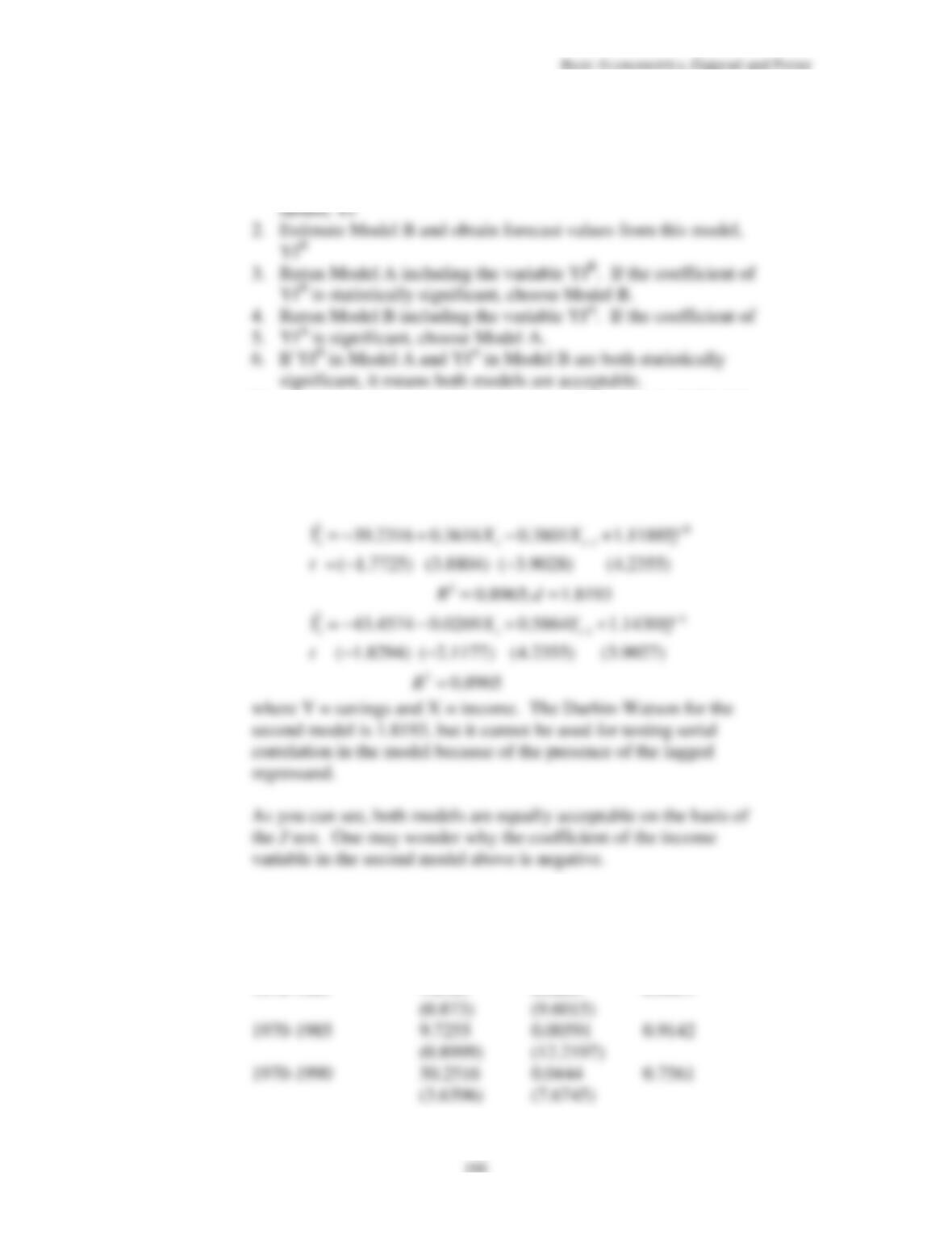
1.Estimate Model B and obtain the estimated values of Y from this
model,
ˆ
B
i
Y
3. Repeat steps 1 and 2, interchanging the roles of A and B.
The regression results are as follows (for convenience the
observation subscript t is omitted):
Based on these results, it seems that Model A is the “correct” model.
13.28
(a) The difference between Model (1) and Model (2) in Exercise
7.19 is that there is one additional explanatory variable in Model (2).
13.29
There are several possibilities. We only consider one, namely, the
Davidson-MacKinnon J test. The steps involved are as follows:
1.
Estimate Model A and obtain the forecast values from this
A
If you carry out the preceding steps, you will find that both Models
are acceptable. So, there is no clear preference here. However, if
you bring in the interest rate, it is quite possible that one of the two
models may be preferable. We give below the regression results
without the interest rate variable.
13.30
The regression results of savings on income are as follows:
Time Period Intercept Slope R
2
1970-1981 1.0161 0.0803 0.9021
Basic Econometrics, Gujarati and Porter
167
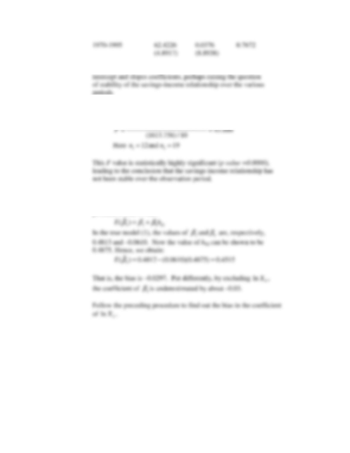
As you can see, there is quite a bit of variability in the estimated
13.31
Follow Eq. (13.10.1). Using the given data, we obtain the following
F value:
13.32
Let us see the effect of excluding
6
ln
X
on the coefficient of the
retained variable ln X
2
. Following the equation given in this
problem, it follows that: