CHAPTER 13
Business Cycle Models with Flexible Prices and Wages
KEY IDEAS IN THIS CHAPTER
1. According to the real business cycle model, business cycles are optimal responses of
3. The Keynesian coordination failure model is based on the existence of strategic
complementarities which give rise to increasing returns to scale at the aggregate level.
4. Increasing returns to scale implies that there can be multiple equilibria. The economy
6. The role of government policy in the coordination failure model could be to produce
optimism, and there may be a role for fiscal policy in smoothing out business cycles.
8. During the financial crisis, there was deficient financial liquidity, and this acts in the
9. The New Monetarist model has important implications for the behavior of the
economy in a liquidity trap.
NEW IN THE FOURTH EDITION
1. The Section on segmented markets was eliminated.
2. A new section on the New Monetarist model has been added, which has some useful
4. All data and graphs have been updated.
5. New end-of-chapter problems.
TEACHING GOALS
Chapter 3 demonstrated there are strong regularities associated with the comovements
among macroeconomic variables. Though business cycles are remarkably similar,
understanding their causes is a difficult task. There are multiple alternative business cycle
models, and students need to understand how these models are different – in terms of
what causes business cycles in these alternative models, and what the policy prescriptions
are. In need not be the case that we want to totally dismiss any business cycle models.
Potentially many models could give us useful insight what business cycles are about.
The models in this chapter are all based on flexible wages and prices. Sometimes these
are called “equilibrium” models, but even models with sticky wages and prices – for
example the New Keynesian model in Chapter 14 – have some notion of equilibrium. It is
important for students to understand, in spite of the fact that much of Keynesian
economics is done with sticky-wage-and-price models, that Keynesian ideas do not
depend on sticky wages and prices.
The last model in this chapter is a New Monetarist model, which is included to capture
specifically some features of the financial crisis, rather than as a general model of
business cycles. The novelty is the idea that financial liquidity is important in financial
crises, and that this requires a different way of thinking about monetary policy.
CLASSROOM DISCUSSION TOPICS
A key idea in this chapter is that a preliminary evaluation of a model’s usefulness
involves fitting the data. It would be good to discuss why this is valid. Might we imagine
models that did not fit the data well but might nevertheless be useful? Do we want the
model to fit all the data? Surely a model intended for the study of business cycles need
not give good predictions about the price of orange juice ten years from now.
Chapter 13: Business Cycle Models with Flexible Wages and Prices
Macroeconomists have been criticized for not foreseeing the financial crisis. Would that
have been feasible? Is forecasting all the macroeconomists do? Point out that an
important goal in macroeconomics is to design models that can be useful for policy
analysis.
Why should we study different business cycle models? Surely they cannot all be correct.
Discuss how policymakers use models to make policy decisions. The models need to be
simple. There can be many factors at work in the real world, but putting these all in one
model may just be confusing.
OUTLINE
1. The Real Business Cycle Model
a) The Workings of the Real Business Cycle Model
i) Persistence of the Solow Residual
ii) Effects of a Persistent Change in Total Factor Productivity
iii) Qualitative and Quantitative Replication of Business Cycle Facts
b) Real Business Cycles and the Behaviour of the Money Supply
i) Cyclical Properties of the Money Supply
(2) Nominal Money Leads Real GDP
ii) Endogenous Money
(2) Central Banks and Price-Level Stabilization
iii) Statistical Causality and True Causality
c) Implications of the Real Business Cycle Model for Government Policy
i) Money is Neutral
ii) Government Spending Based on Optimal Provision of Public Goods
iii) Other Policy Goals
(1) The Friedman Rule
(2) The Smoothing of Tax Distortions
d) Critique of the Real Business Cycle Model
e) Business Cycle Models and the Great Depression in Canada (Macroeconomics in
Action 11.1)
f) Recessions in the Mid-1970s and the Early 1980s (Theory Confronts the Data
11.1)
2. A Keynesian Coordination Failure Model
a) The Workings of the Model
i) Coordination Failures
ii) Strategic Complementarities
iii) Multiple Equilibria
iv) Increasing Returns to Scale
b) The Coordination Failure Model: An Example
i) The Downward-Sloping Goods Supply Curve
c) Predictions of the Coordination Failure Model
i) Properties of “Good” and “Bad” Equilibria
ii) The Coordination Failure Model and Business Cycle Facts
d) Policy Implications of the Coordination Failure Model
i) Achieving a Single Equilibrium
ii) Does Policy Improve Performance?
e) Regional Differences in Business Cycle Activity in Canada (Macroeconomics in
Action 11.2)
f) Critique of the Coordination Failure Model
3. A New Monetarist Model: Financial Crises and Deficient Liquidity
a) The model – an extension of the monetary intertemporal model
b) A reduction in financial liquidity during the financial crisis – effects in the model
c) Policy response to a reduction in financial liquidity
d) Deficient financial liquidity, excess reserves, and the liquidity trap
TEXTBOOK QUESTION SOLUTIONS
Problems
1. The effects in the goods and labor markets are identical to what we considered in
Chapter 11. Output increases, the real interest rate rises, consumption and investment
fall, employment rises, and the real wage falls. What we need to add to the Chapter 11
2. We already know that permanent increases in total factor productivity are consistent
with all of the business cycle facts. As developed in the answer to problem 1, above,
we noted that temporary increases in government spending were not consistent with
3.
11. Here, we need to add the effects in the money market. Since output increases
and the real interest rate increase, the net effect on money demand is ambiguous,
so the price level could rise or fall.
b) From Chapter 11, we know that this shock causes investment to increase, there is
an ambiguous effect on consumption (income increases and the real interest rate
productivity are countercyclical in the model but procyclical in the data. .
4. If the money supply were the only variable that shifts the economy between the bad
and good states, the monetary authority would need to increase the money supply
only if the economy starts out in the bad state. However, once the good state is
reached, there is no further need to make any changes in the money supply.
5. This shock acts to shift the labor supply curve to the right which, when we construct
the output supply curve, implies a shift to the left in that curve. As well, because there
is an increase in the demand for consumption goods, the output demand curve shifts
to the right. As shown in Figure 13.1, output in the good equilibrium increases, and
the real interest rate is lower in the good equilibrium. Thus, in the good equilibrium,
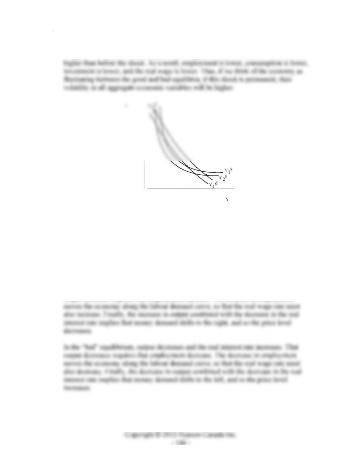
Instructor’s Manual for Macroeconomics, Fourth Canadian Edition
employment is higher, consumption is higher, investment is higher, and the real wage
is higher. However, in the bad equilibrium, output is lower and the real interest rate is
Figure 13.1
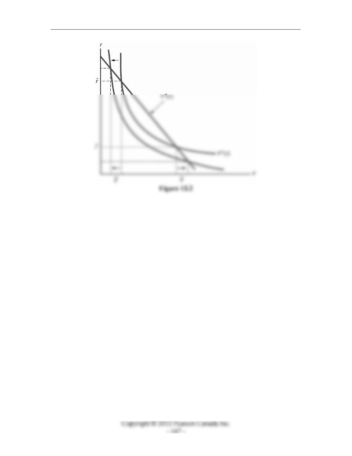
6. The permanent increase in government spending does not affect the aggregate
demand curve, because the increase in government spending generates an
approximately equal decrease in consumption. The implied increase in taxes shifts the
labour supply curve to the right. In the coordination failure model, this produces a
leftward shift in aggregate supply. Recall that the labour demand curve is upward
sloping and steeper than the labour supply curve. A leftward shift in aggregate supply
is depicted in Figure 13.2, below.
In the “good” equilibrium, output increases and the real interest rate decreases. That
output increases requires that employment increase. The increase in employment
Chapter 13: Business Cycle Models with Flexible Wages and Prices
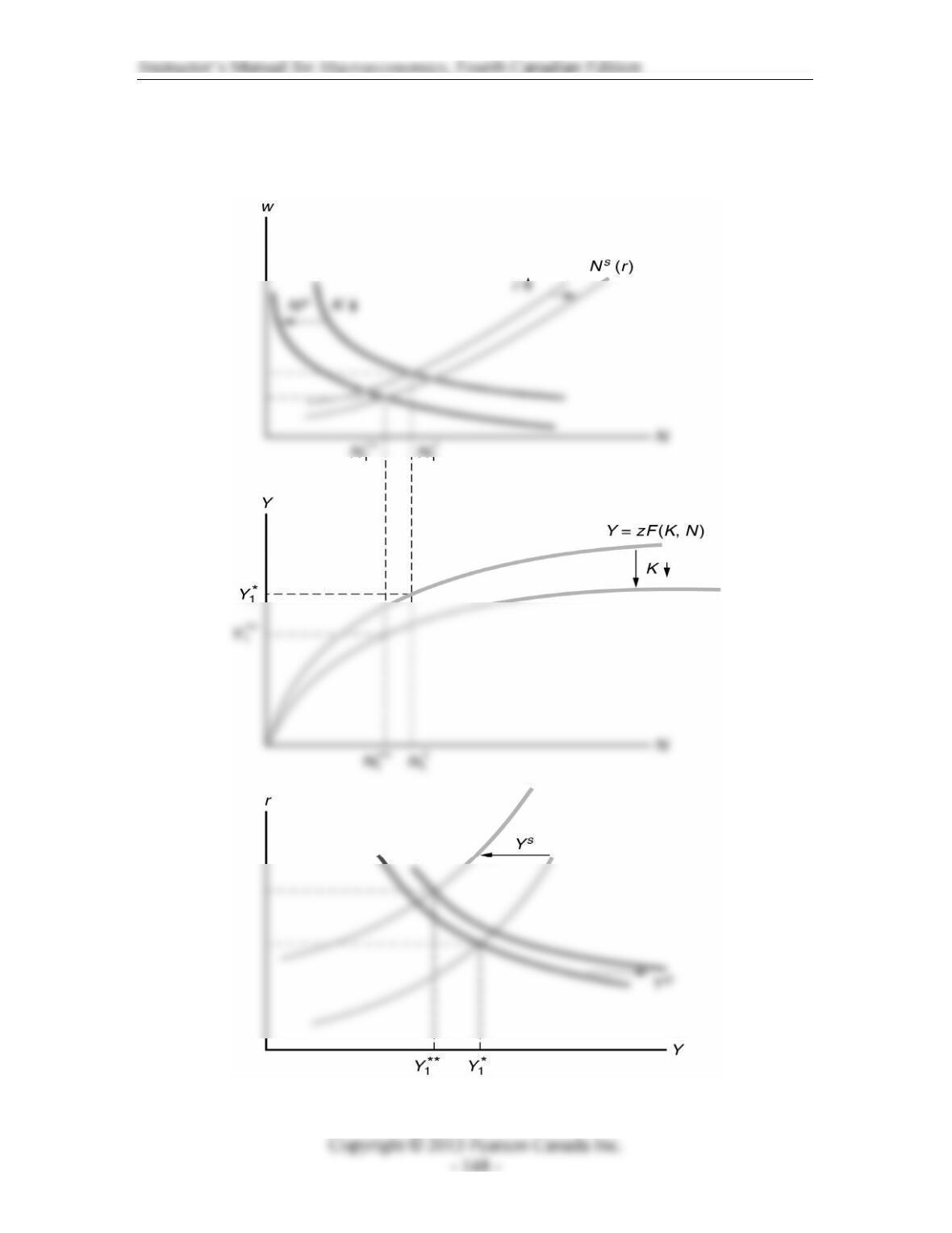
7. The effects of the decrease in the capital stock depend on the specific model we are
working with. The effect of the decrease in capital in the real business cycle is
depicted in Figure 13.3, below.
Figure 13.3
Chapter 13: Business Cycle Models with Flexible Wages and Prices
The real interest rate unambiguously increases. The diagram depicts a case in which
real output decreases. In this case, the demand for money unambiguously decreases,
8. a) In the real business cycle model, what the central bank should do in response to a
b) In the coordination failure model, money is neutral, just as in the real business
cycle model, unless money plays the role of a “sunspot” variable. In that case,
central bank actions mean something to private sector economic agents, and the
9. In the New Monetarist model, if there is deficient financial liquidity, then a tax cut
financed by an increase in the quantity of nominal government bonds, B, will increase
the quantity of liquid financial assets, a. This shifts the output demand curve to the

Instructor’s Manual for Macroeconomics, Fourth Canadian Edition
Figure 13.4
10. Whether there is a liquidity trap or not, the tax cut financed by a government bond
11. If there is deficient financial liquidity, then quantitative easing – an increase in M
matched by a decrease in k(r) – gives the same effects as in Figure 13.16 in the