Compound Options
13.23
• Compound option parameters
0
V
1
I
2
I
1
T
2
T
r
σ
$32.43
$10
$30
1
3
0.06
0.5
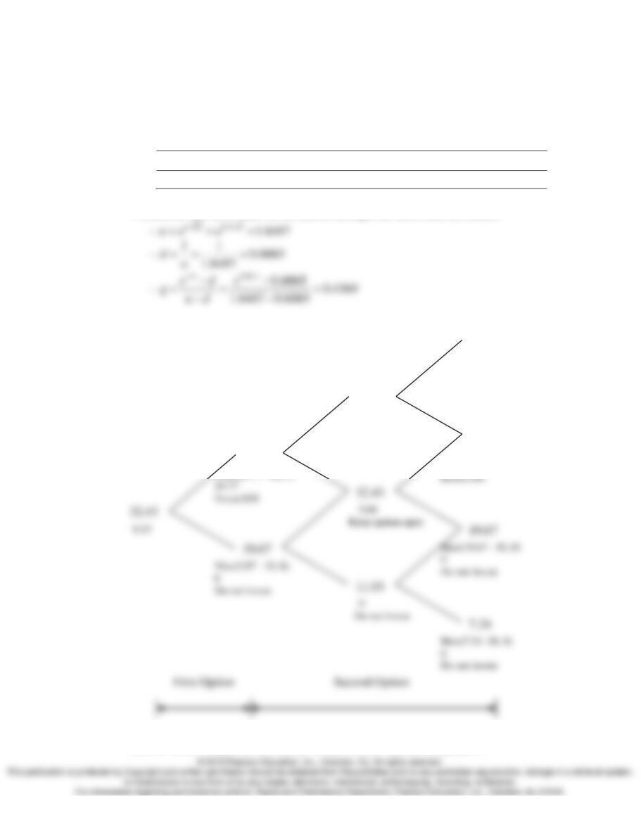
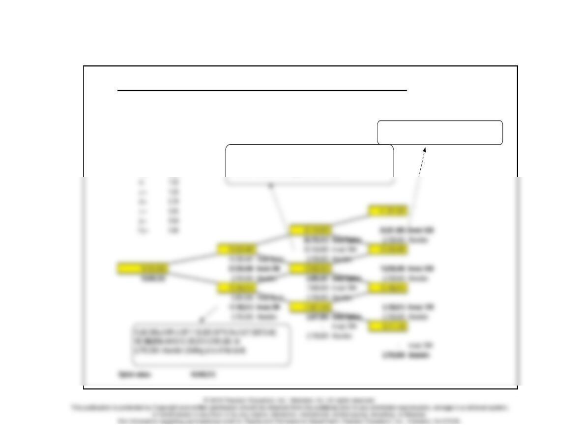
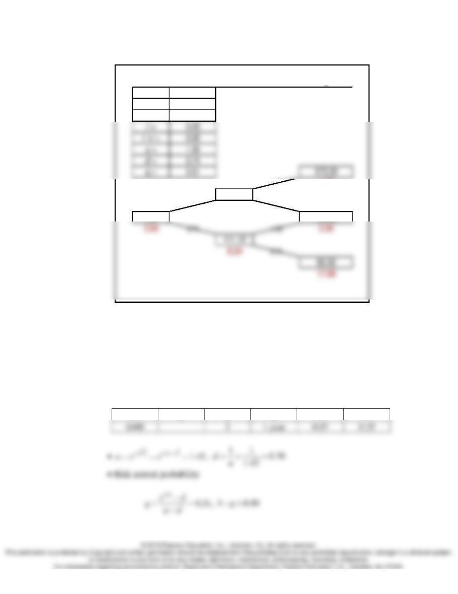
• Decision tree for a scale-down option through one-year time increment.
19.67
Max(3.97 – 10, 0)
32.43
32.43
11.93
19.67
Max(19.67 – 30, 0)
7.24
Max(7.24 –30, 0)
ENPW is $8.13 and this exceed the initial cost $5. Initiate the phase I.
53.47
Max(29.77 – 10, 0)
88.15
59.90
Keep option open
53.47
Max(53.47 – 30, 0)
23.47
145.34
Max(145.34 – 30, 0)
115.34
Invest $30
13.24
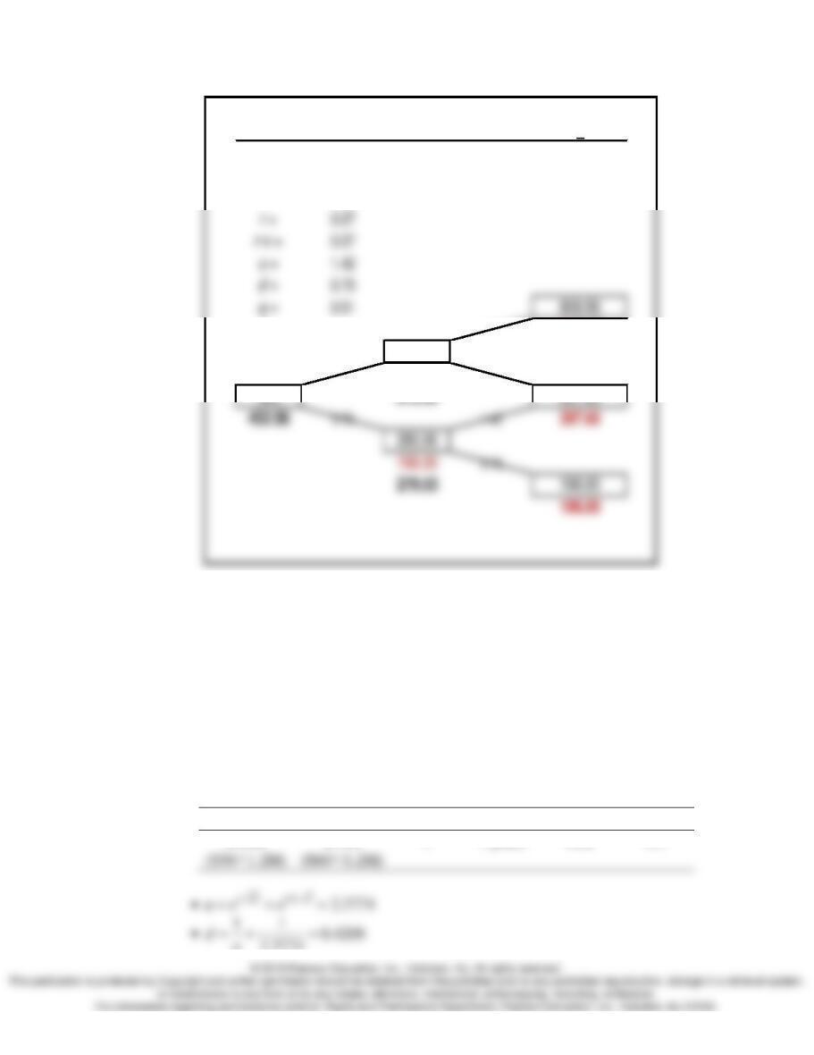
• Option parameters
0
V
1
I
2
I
T
r
σ
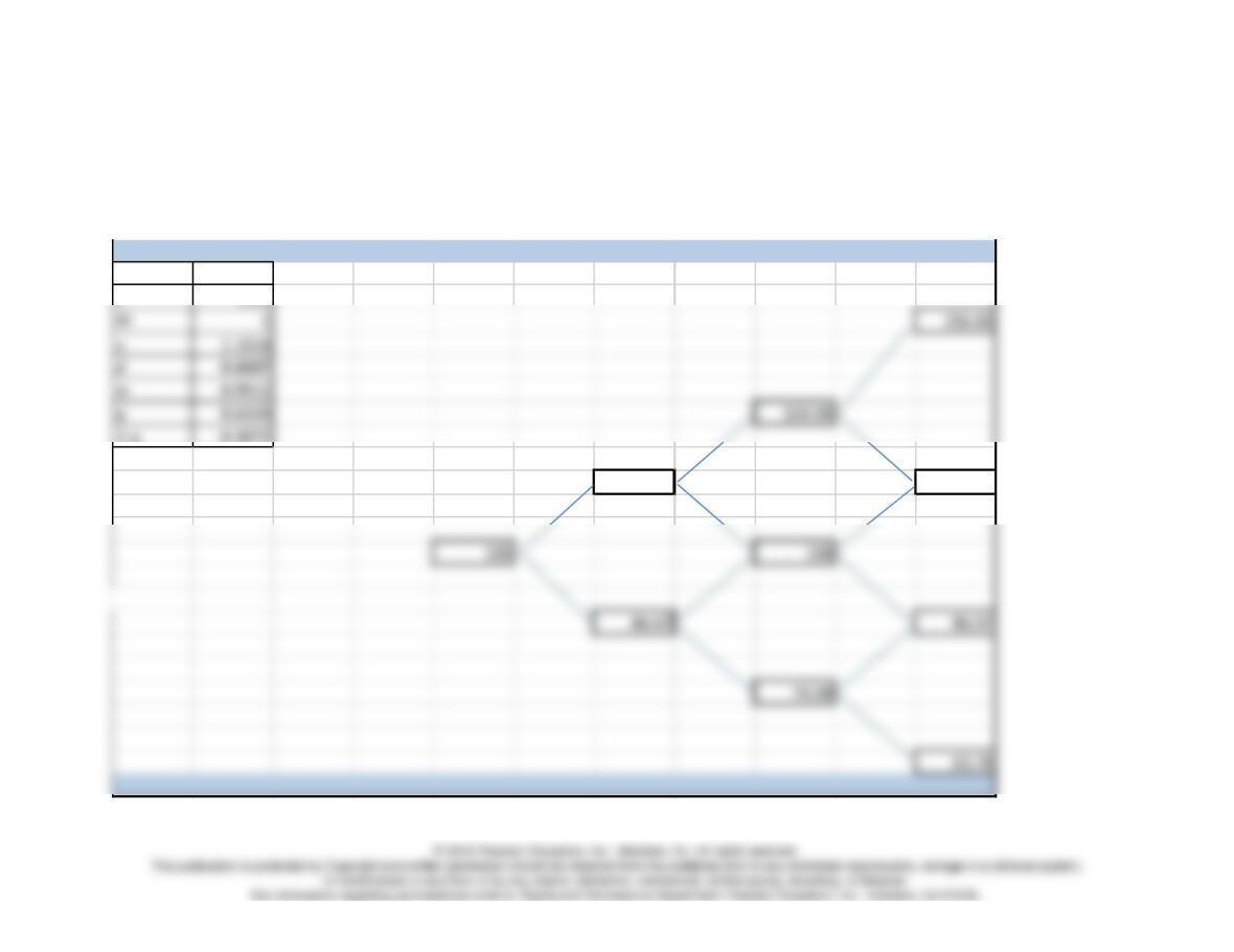
Phase 1 Phase 2
0 1 2 3
I= 3,000,000 12,000,000 12,000,000
volatility= 0.25
r = 0.05
T = 3.00
29,281,500=MAX(41,281,500–12,000,000, 0)
2,700,000: Abandon (Selling price of the land)
20,735,312=EXP(–0.05*1)*(29,281,500*0.54+13,038,496*0.46)
20,150,065=MAX(32,150,065–12,000,000, 0)
2,700,000: Abandon (Selling price of the land)
13.25
Event tree: Binomial lattice
σ0.15 0 1 2 3
r0.05
1-q 0.3672
116.18 116.18
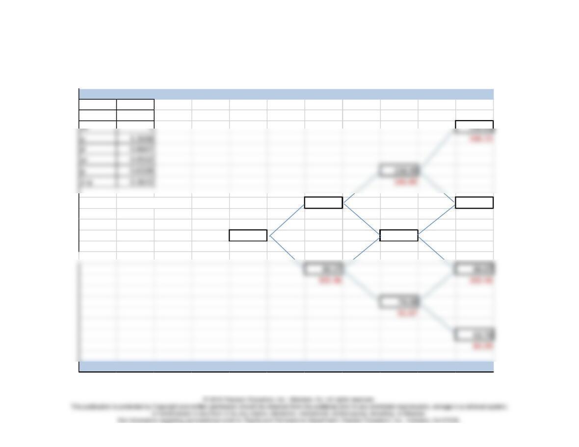
(a) Contract Option: Best strategy – Contract now – Option value = $15
σ0.15 0 1 2 3
r0.05
Contract now. 116.18 116.18
129.57 129.57
100 100
115 115
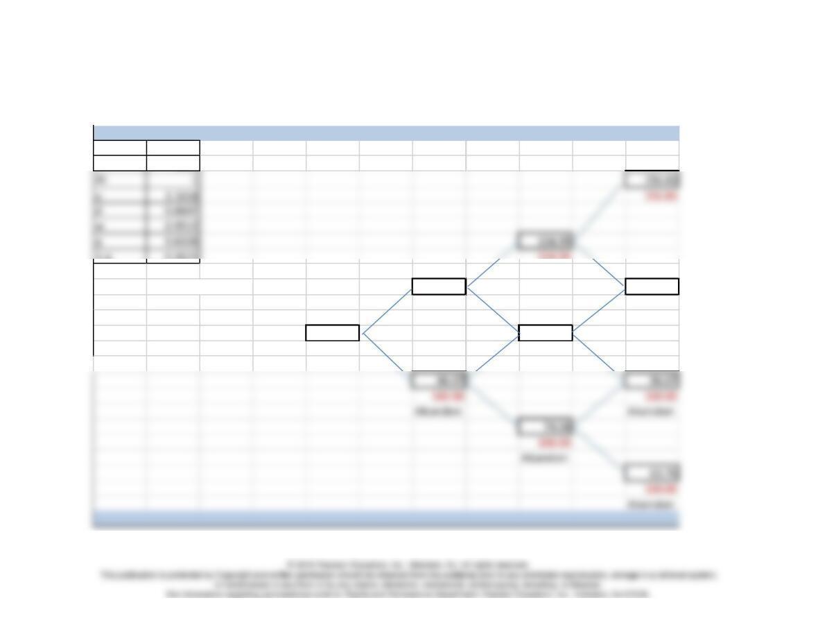
(b) Abandonment Option: Option value = $5.89
σ0.15 0 1 2 3
r0.05
1-q 0.3672 134.99
Contract now. 116.18 116.18
117.88 116.18
100 100
105.89 104.86
(c) Expansion Option: Option value = $12.82
σ0.15 0 1 2 3
r0.05
∆t1156.83
116.18 116.18
132.94 131.04
Expand
(d) Combined Options: Option value = $17.25
σ0.15 0 1 2 3
r0.05
∆t1156.83
134.99
116.18 146.49 116.18
132.94 156.46 131.04
117.88 116.18
100 129.57 100 129.57
Short Case Studies
ST 13.1
(a)
V
0
100 V
1
122 V
1
82
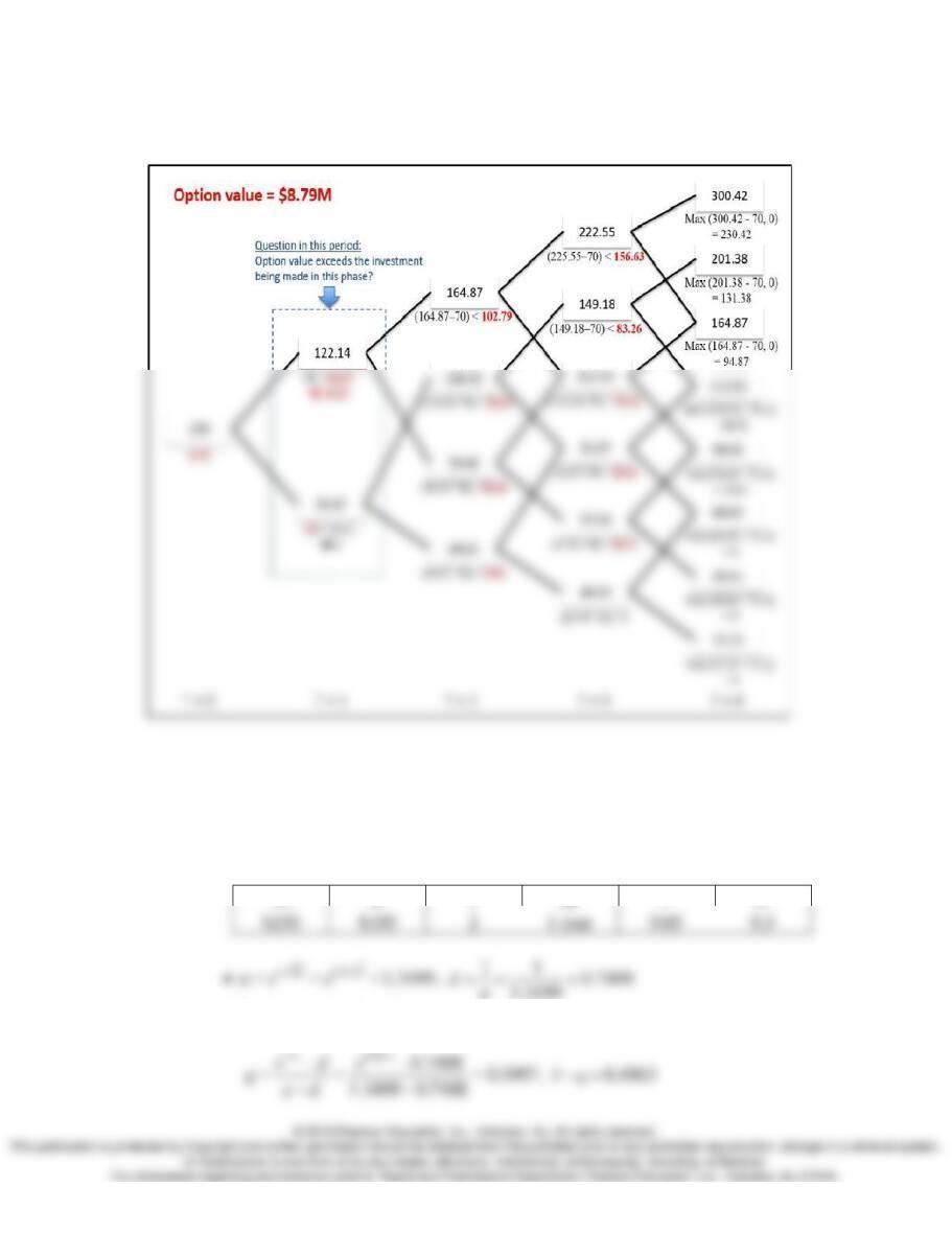
u1.2214028 300
d0.8187308 230
q0.6037315 $223
$165 165
u1.3498588 $105 95
d0.7408182
q0.5270886 $122 $122
1-q 0.4729114 $17.46 $57
e(-rt) 0.9512294 90
$90 20
$33
67 50
$111
70
(b)
ST 13.2
(a) American put option value
• Option parameters
V
0
K
T
t∆
r
σ
1.3499
• Risk neutral probability
0 1 2
v = 0
K =
100
σ =
0.3
1.35 0.00
202.48
1.35 0.00 0.74
150 150.00
∴ American put option value = $3.84 (In our example, dividend rate (v) = 0.)
(b) Expansion Option value
• Option parameters
V
0
K
T
t∆
r
σ
0 1 2
σ =
0.35
1.42
1040.50
568.00
1.42
658.80
0.70
∴ Expansion option value = $452.58
ST 13.3
(a) Since $4 M is lower than the option price, it is a good investment for Merck
Co.
• To give a range for the option value, first using one period lattice.
V
0
K
T
t∆
r
σ
$36M
$72M
3
3 years
0.06
0.5
2.3774
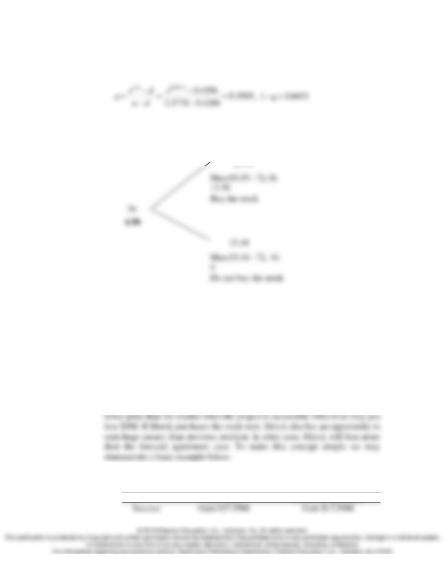
• Risk neutral probability
• One period lattice and option price: 4.50M
• Through the B-S model, the option price should be $6.54M.
Note: We can think that the price from the one step binomial tree is the lower bound
and B-S is the upper bound. So the option price is definitely higher than the
suggested price.
(b) By buying the aforesaid agreement, Merck has a chance to buy Genetics with a
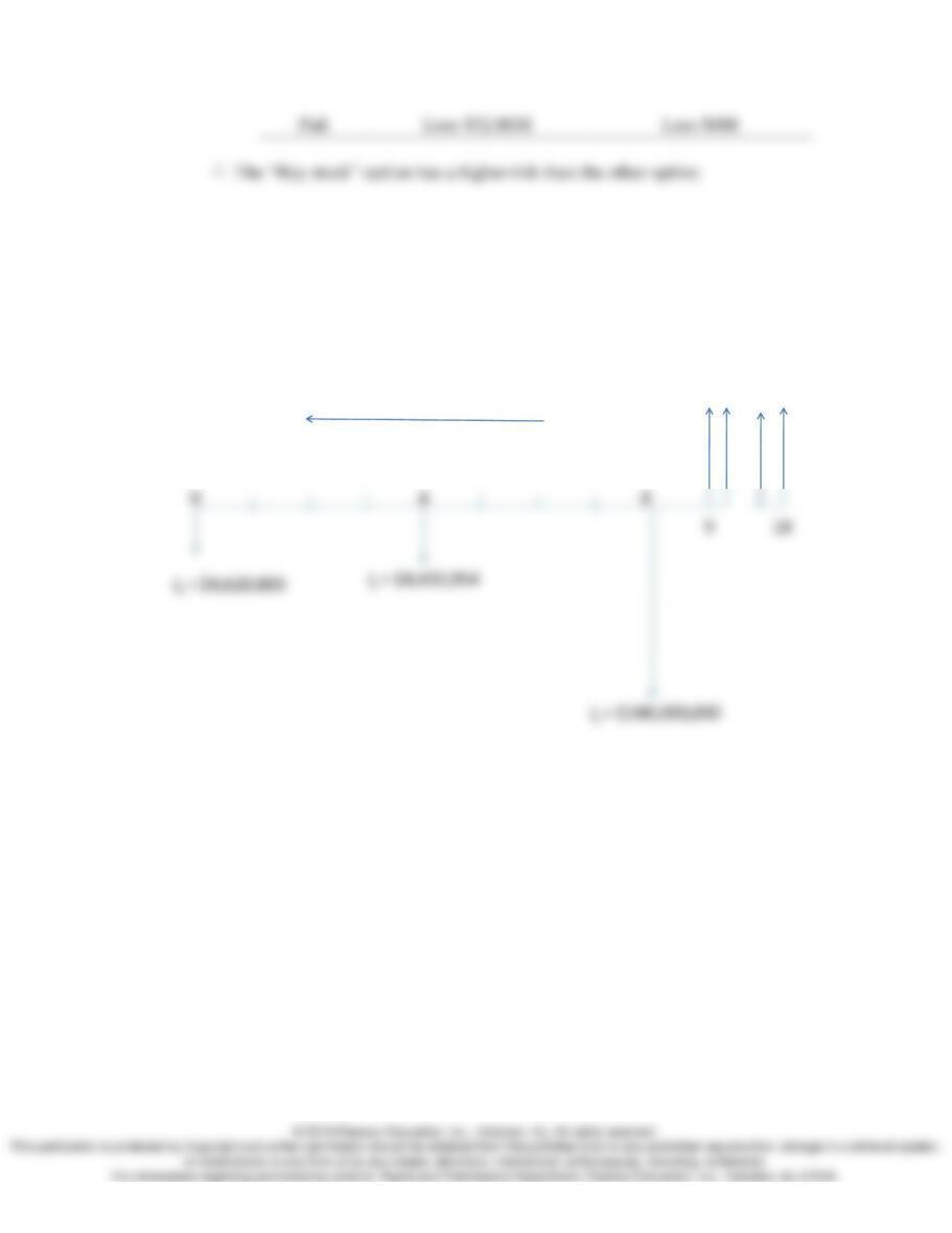
• Profit/loss analysis
Buy stock
Aforesaid agreement
ST 13.4
0
= $4,435,954
2
= $100,000,000
R&D
Phase
Development
Phase
Manufacturing
Phase
V
8
= $144,821,558
V
0
= $58,490,998
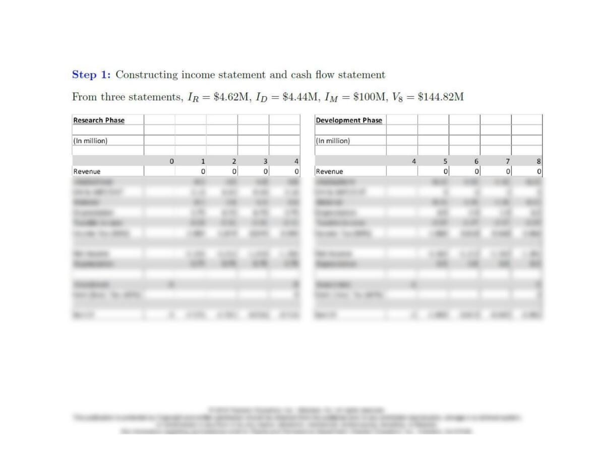
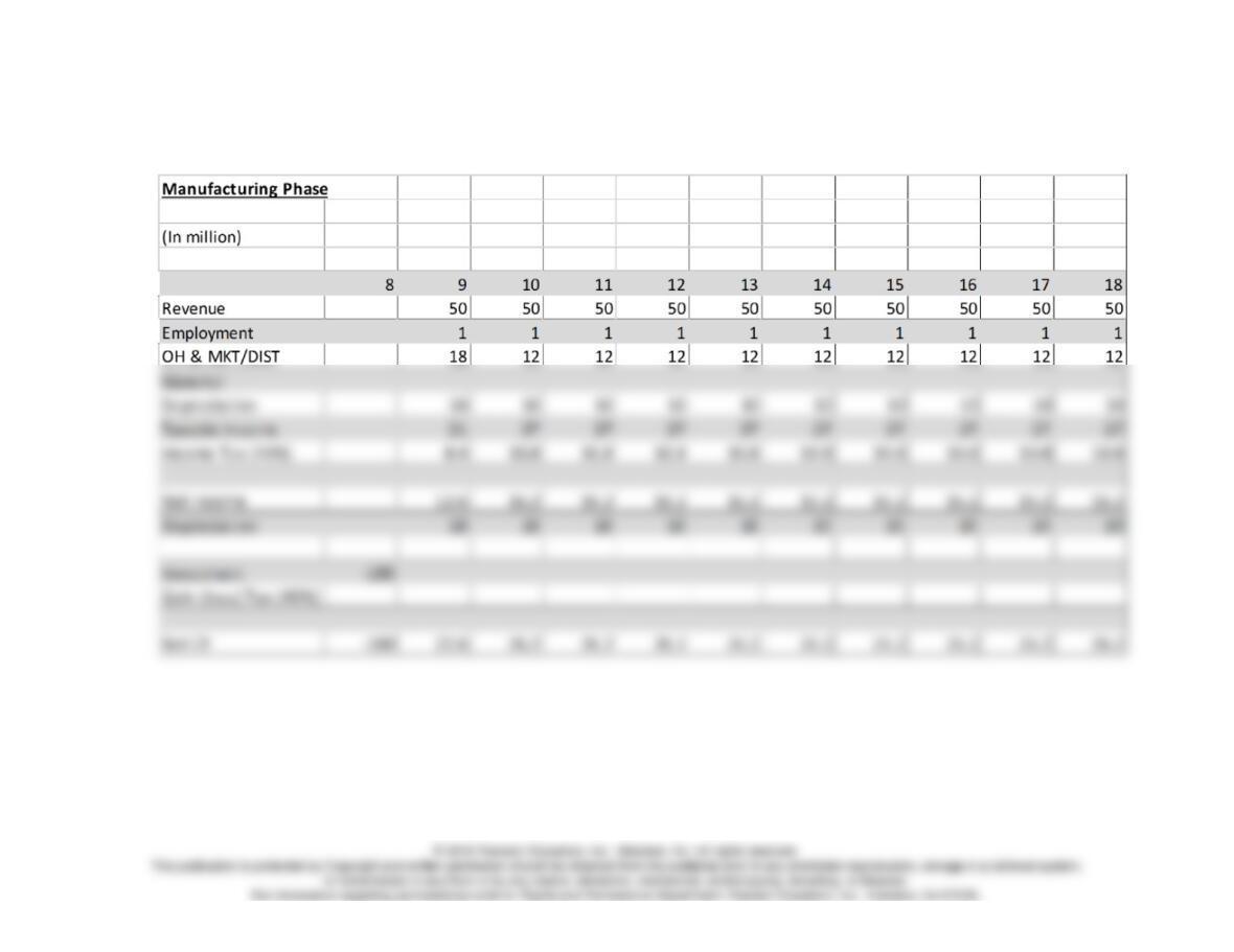
(continued)
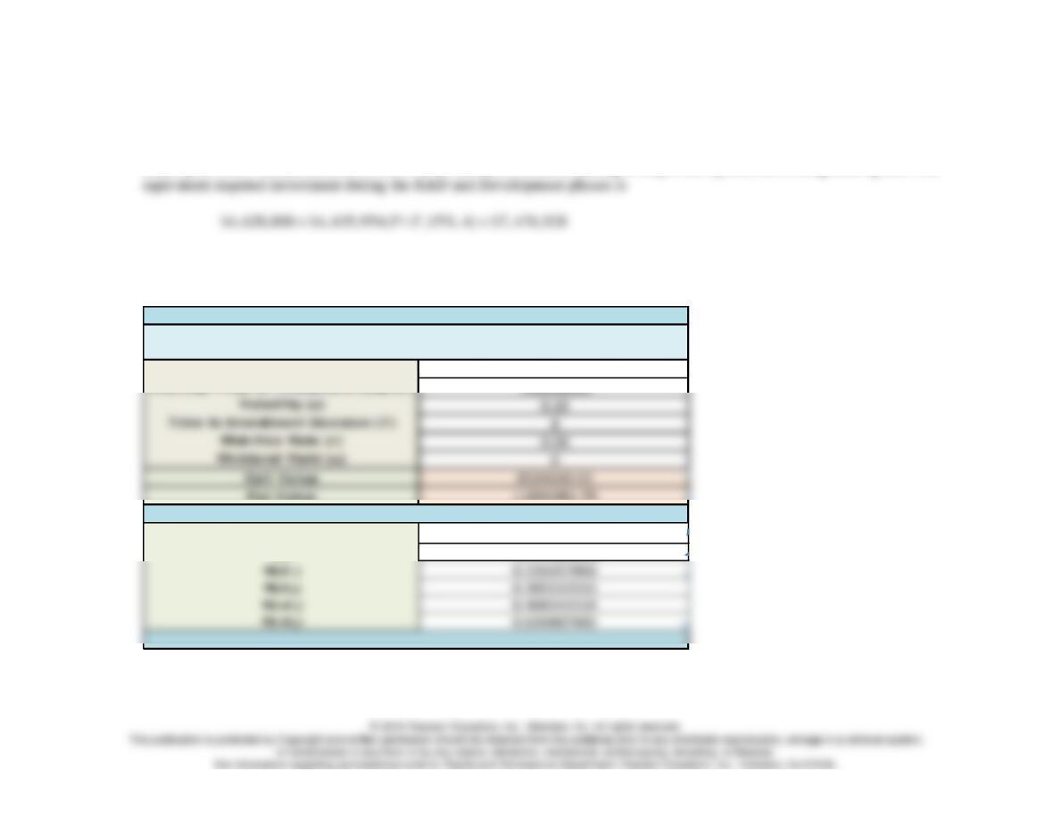
• Once students generate the cash flows in each phase of the project, ask them to determine whether or not it is worth investing
$4,620,800 at n = 0, and $4,435,954 at n = 4. In this case, we are assuming a simple call option, not a compound option. The
which exceeds the option value calculated by the B-S Model ($8,504,641), so we may suggest that the firm may initiate both
R&D and Development activities.
Stock price (S
0
) or Project Value (V
0
)
58490998
Exercise Price or Investment Cost (K)
100000000
Put Value
11891981.79
d
1
0.079437969
d
2
–0.344826099
Black-Scholes Model
However, this is not a simple option.