CHAPTER 13 | Aggregate Demand and
Aggregate Supply Analysis
Brief Chapter Summary and Learning Objectives
This book takes a fresh approach to the standard aggregate demand and aggregate supply model. There is
no good, simple alternative to using the AD-AS model when explaining movements in the price level and
real GDP. But many instructors are dissatisfied with relying exclusively on the AD-AS model. The key
problem, of course, is that AD-AS is a static model that attempts to account for dynamic changes in real
GDP and the price level. The authors’ approach retains the basics of the AD-AS model but makes it more
accurate and useful by making it more dynamic. The authors emphasize two points:
1. Changes in the position of the short-run (upward-sloping) aggregate supply curve depend mainly
13.1 Aggregate Demand (pages 816–824)
Identify the determinants of aggregate demand and distinguish between a movement
along the aggregate demand curve and a shift of the curve.
13.2 Aggregate Supply (pages 824–830)
Identify the determinants of aggregate supply and distinguish between a movement along
CHAPTER 13 | Aggregate Demand and Aggregate Supply Analysis 301
13.3 Macroeconomic Equilibrium in the Long Run and the Short Run
(pages 830–836)
Use the aggregate demand and aggregate supply model to illustrate the difference
between short-run and long-run macroeconomic equilibrium.
▪ In long-run macroeconomic equilibrium, the aggregate demand and short-run aggregate
13.4 A Dynamic Aggregate Demand and Aggregate Supply Model
(pages 837–843)
Use the dynamic aggregate demand and aggregate supply model to analyze
macroeconomic conditions.
▪ To make the aggregate demand and aggregate supply model dynamic, we assume that:
Appendix: Macroeconomic Schools of Thought (pages 851–854)
Compare macroeconomic schools of thought.
Key Terms
Aggregate demand (AD) curve, p. 816. A
curve that shows the relationship between the
price level and the quantity of real GDP
demanded by households, firms, and the
government.
Monetary policy, p. 819. The actions the
Federal Reserve takes to manage the money
supply and interest rates to achieve
macroeconomic policy objectives.
302 CHAPTER 13 | Aggregate Demand and Aggregate Supply Analysis
Key Terms—Appendix
Keynesian revolution, p. 851. The name given
to the widespread acceptance during the 1930s
and 1940s of John Maynard Keynes’s
macroeconomic model.
New classical macroeconomics, p. 852. The
macroeconomic theories of Robert Lucas and
others, particularly the idea that workers and
firms have rational expectations.
Chapter Outline
The Fortunes of Delta Airlines Follow the Business Cycle
Delta Airlines has grown into the world’s largest airline, earning more than $40 billion in revenue
worldwide in 2015. Delta’s fortunes and the fortunes of the other U.S. airlines are dependent on the ups
13.1
Aggregate Demand (pages 816–824)
Learning Objective: Identify the determinants of aggregate demand and distinguish
between a movement along the aggregate demand curve and a shift of the curve.
The aggregate demand and aggregate supply model explains short-run fluctuations in real GDP and
the price level. The aggregate demand (AD) curve shows the relationship between the price level
A. Why Is the Aggregate Demand Curve Downward Sloping?
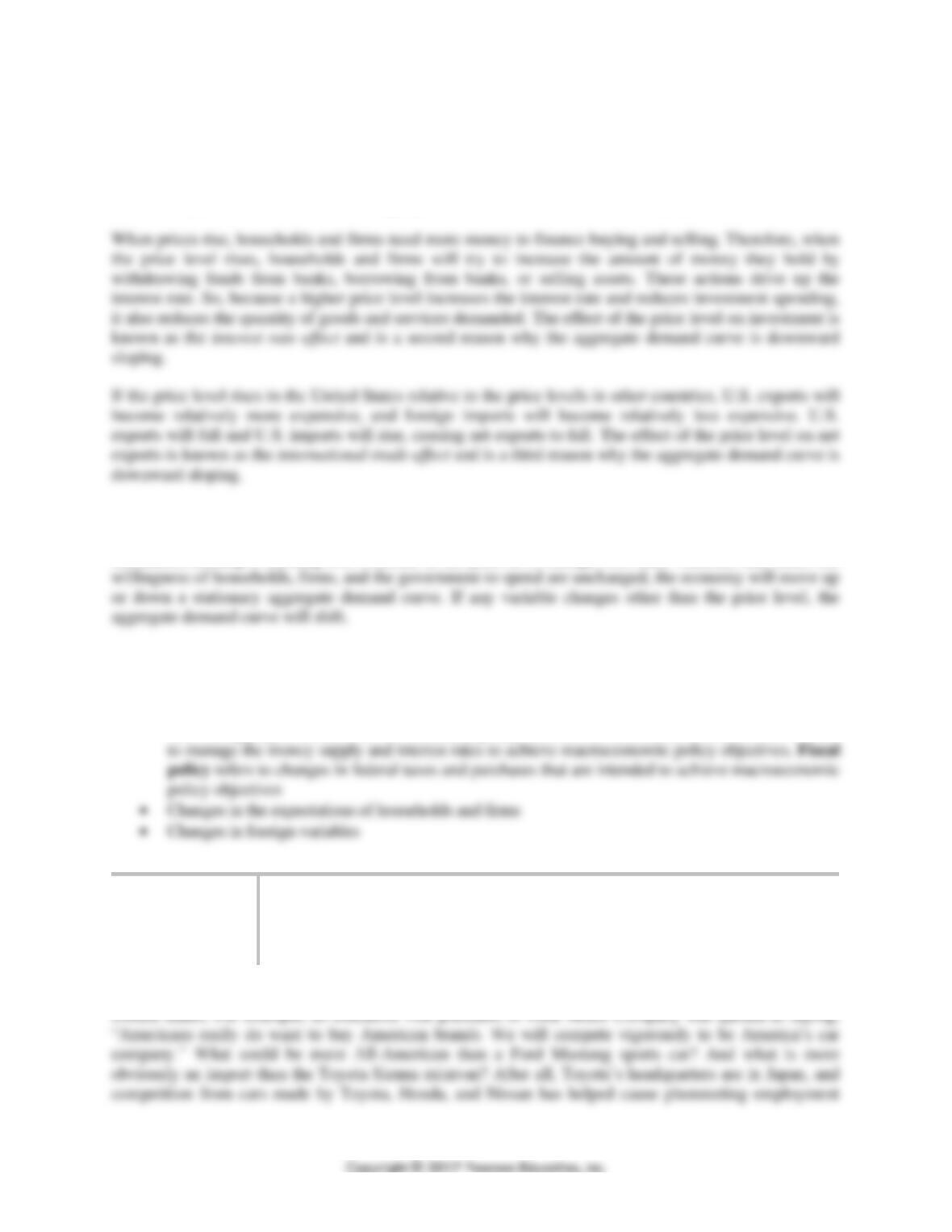
GDP has four components: consumption (C), investment (I), government purchases (G), and net exports
(NX). If we let Y stand for GDP, we can write:
CHAPTER 13 | Aggregate Demand and Aggregate Supply Analysis 303
The aggregate demand curve is downward sloping because a fall in the price level increases the quantity
of real GDP demanded. Current income is the most important variable determining consumption by
households. But consumption also depends on wealth. When the price level rises, the real value of
household wealth declines and so will consumption. The effect of the price level on consumption is called
the wealth effect and is one reason the aggregate demand curve is downward sloping.
B. Shifts of the Aggregate Demand Curve versus Movements along It
The aggregate demand curve tells us the relationship between the price level and the quantity of real GDP
demanded, holding everything else constant. If the price level changes but other variables that affect the
C. The Variables That Shift the Aggregate Demand Curve
Three variables shift the aggregate demand curve:
• Changes in government policies. The federal government uses monetary policy and fiscal policy to
shift the aggregate demand curve. Monetary policy refers to the actions the Federal Reserve takes
Extra Making
the
Connection
In a Global Economy, How Can You Tell the Imports from the
Domestic Goods?
Some U.S. firms appeal to the patriotism of U.S. consumers by urging them to buy products made in the

304 CHAPTER 13 | Aggregate Demand and Aggregate Supply Analysis
and production at Ford and the other U.S. “Big Three” automakers. But things are not so simple in the
modern global economy. While Ford’s Mustang is assembled in Flat Rock, Michigan, Toyota’s Sienna is
not assembled in Japan but in Princeton, Indiana. Most firms that sell products, such as automobiles, that
have many parts, purchase those parts from suppliers who may be located anywhere in the world.
According to the U.S. National Highway Traffic Safety Administration, 65 percent of the content of the
Ford Mustang was produced by Ford itself or by firms located in the United States or Canada. The other
35 percent of the content was imported from firms located in other countries. By contrast, 90 percent of
Question
Suppose that a consumer in Germany buys a Ford Mustang for a price of $30,000. Do U.S. exports
increase by $30,000? Briefly explain.
Answer
Teaching Tips
The end of the chapter in the main text includes a special category of exercises titled Real-Time Data
Exercises. These exercises help students become familiar with a key data source, learn how to locate data,
13.2
Aggregate Supply (pages 824–830)
Learning Objective: Identify the determinants of aggregate supply and distinguish
between a movement along the short-run aggregate supply curve and a shift of the
curve.
A. The Long-Run Aggregate Supply Curve
Because changes in the price level do not affect the number of workers, the capital stock, or technology in
CHAPTER 13 | Aggregate Demand and Aggregate Supply Analysis 305
B. The Short-Run Aggregate Supply Curve
The short-run aggregate supply curve is upward sloping because, over the short run, as the price level
increases the quantity of goods and services firms are willing to supply increases. The main reason firms
C. Shifts of the Short-Run Aggregate Supply Curve versus Movements along It
If the price level changes but other variables are unchanged, the economy will move up or down a
stationary aggregate supply curve. If any variable other than the price level changes, the aggregate supply
curve will shift.
D. Variables That Shift the Short-Run Aggregate Supply Curve
The most important variables that cause the short-run aggregate supply curve to shift are:
• Increases in the labor force and in the capital stock
Extra Solved Problem 13.2
Sticky Prices and Wages
Changes in real GDP occur in response to price level changes over short periods of time when input
prices rise more slowly than output prices. Because real GDP responds to changes in the price level in the
short run, the short–run aggregate supply curve is upward sloping. Economists use the phrases “sticky
wages” and “sticky prices” to refer to the slow response of wages and other input prices, as well as some
output prices, to price level changes. To help understand why prices and wages may be sticky, let’s use

306 CHAPTER 13 | Aggregate Demand and Aggregate Supply Analysis
Solving the problem
Step 1: Review the chapter material.
Step 2: Explain why Bill might increase the price and output of glue during 2018 but
reduce the output of glue to its previous (2017) level in 2019.
The price level increase means that other output prices have risen. As a result, suppose that
Step 3: Explain why Bill might choose not to raise the price of glue during 2018 but would
increase the output of glue during 2018 and reduce the production of glue to its
former (2017) level in 2019.
Bill might choose this option if he is not sure if the increase in the price level will be
sustained. If he raises prices in 2018, he risks losing customers to other glue sellers. In
13.3
Macroeconomic Equilibrium in the Long Run and the Short Run
(pages 830–836)
Learning Objective: Use the aggregate demand and aggregate supply model to
illustrate the difference between short-run and long-run macroeconomic equilibrium.
We can use the aggregate demand and aggregate supply model to analyze changes in real GDP and the
price level. In the long run, the short-run aggregate supply curve and the aggregate demand curve
A. Recessions, Expansions, and Supply Shocks
Assume that:
1. The economy has not been experiencing any inflation. The price level is 110 and is expected to
stay at that level.
2. The economy is not experiencing any long-run growth.
CHAPTER 13 | Aggregate Demand and Aggregate Supply Analysis 307
Though unrealistic, these assumptions allow us to understand the key ideas of the aggregate demand and
aggregate supply model. Assume that rising interest rates reduce investment and cause the aggregate
demand curve to shift to the left, resulting in a recession. The recession will eventually end because there
If many firms become more optimistic about the future profitability of new investment, the resulting
increase in investment shifts the AD curve to the right. Firms will operate beyond their normal capacity,
and some workers who would ordinarily be structurally or frictionally unemployed are employed. An
automatic mechanism will bring the economy back from a short-run equilibrium beyond potential GDP.
Extra Solved Problem 13.3
Short-Run and Long-Run Equilibrium
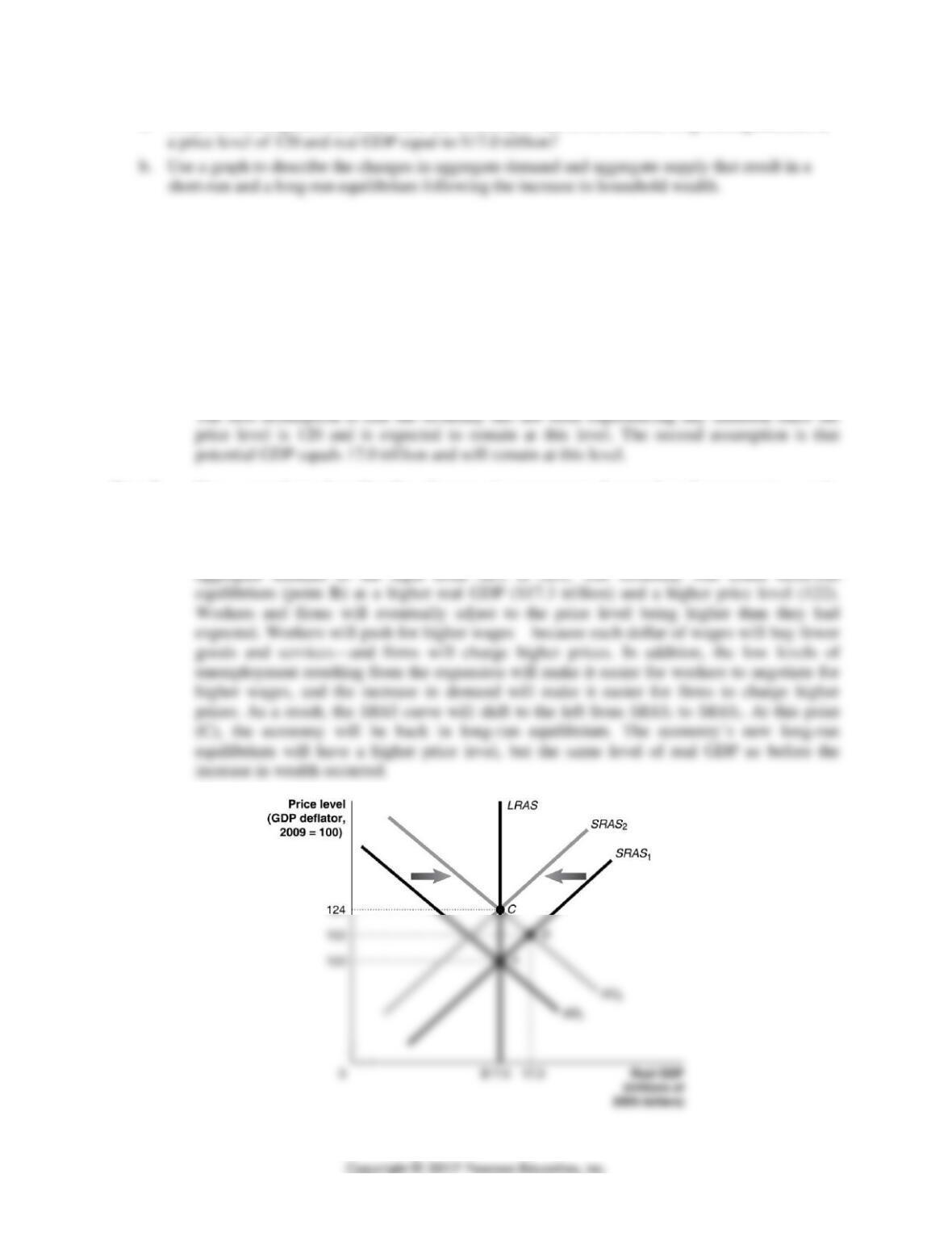
The following graph illustrates an economy in long-run equilibrium at a price level of 120 and real GDP
of $17.0 trillion. Assume that an increase in real estate prices raises household wealth.
308 CHAPTER 13 | Aggregate Demand and Aggregate Supply Analysis
a. What two assumptions are used when the economy is said to be in initial long-run equilibrium at
Solving the Problem
Step 1: Review the chapter material.
This problem is about the relationship between short-run and long-run macroeconomic
equilibrium, so you may want to review the section “Macroeconomic Equilibrium in the
Long Run and the Short Run,” which begins on page 830 in the textbook.
Step 2: Explain the two assumptions used when the economy is said to be in initial long–
run equilibrium.
Step 3: Use a graph to describe the changes in aggregate demand and aggregate supply
that result in a short-run and a long-run equilibrium following the increase in
household wealth.
The increase in wealth will increase consumption. This increase will cause a shift in
CHAPTER 13 | Aggregate Demand and Aggregate Supply Analysis 309
Extra Making
the
Connection
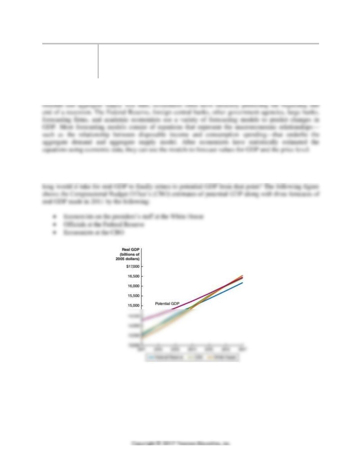
How Long Does it Take to Return to Potential GDP?
Economic Forecasts Following the Recession of 2007–2009
Making accurate macroeconomic forecasts is difficult. As we have seen, many factors can cause
aggregate demand or aggregate supply to shift. Because it is challenging to predict how much aggregate
Most economists agree that an automatic mechanism brings the economy back to potential GDP in the
long run. But how long is the long run? When the recession of 2007–2009 ended in June 2009, real GDP
was far from potential GDP. In 2015, real GDP still remained nearly 4 percent below potential GDP. How
The forecasts of the White House and the CBO agreed that real GDP would not return to potential GDP
until 2016. The projections of the Federal Reserve were even more pessimistic, with real GDP remaining
below potential GDP in 2017. These forecasts indicate how severe the 2007–2009 recession was because
real GDP was not expected to return to potential GDP until seven years after the end of the recession.
Prior to the 2007–2009 recession, the recession of 1981–1982 had been the most severe since the Great
Depression. Yet it took less than three years after the end of that recession for real GDP to return to
potential GDP.
310 CHAPTER 13 | Aggregate Demand and Aggregate Supply Analysis
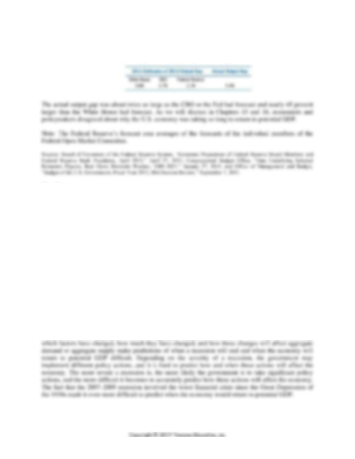
Economists refer to the percentage difference between real GDP and potential GDP as the output gap.
The table shows the 2011 forecasts of the output gap and the actual output gap as of the end of June 2013.
Question
In early 2009, Christina Romer, who was then the chair of the Council of Economic Advisers, and Jared
Bernstein, who was then an economic adviser to Vice President Joseph Biden, forecast how long they
expected it would take for real GDP to return to potential GDP, assuming that Congress passed fiscal
policy legislation proposed by President Obama:
It should be understood that all of the estimates presented in this memo are subject to significant
margins of error. There is the obvious uncertainty that comes from modeling a hypothetical
package rather than the final legislation passed by the Congress. But there is the more
fundamental uncertainty that comes with any estimate of the effects of a program. Our estimates
of economic relationships ... are derived from historical experience and so will not apply exactly
in any given episode. Furthermore, the uncertainty is surely higher than normal now because the
current recession is unusual both in its fundamental causes and its severity.
Why would the causes of a recession and its severity affect the accuracy of forecasts of when the
economy would return to potential GDP?
Source: Christina Romer and Jared Bernstein, The Job Impact of the American Recovery and Reinvestment Plan, January 9,
2009, p. 2.
Answer
Many factors cause aggregate demand or aggregate supply to shift, and the difficulty of determining

CHAPTER 13 | Aggregate Demand and Aggregate Supply Analysis 311
13.4
A Dynamic Aggregate Demand and Aggregate Supply Model
(pages 837–843)
Learning Objective: Use the dynamic aggregate demand and aggregate supply model
to analyze macroeconomic conditions.
The basic aggregate demand and aggregate supply model leads to some misleading results because of
these assumptions: (1) the economy does not experience continuing inflation, and (2) the economy does
A. What Is the Usual Cause of Inflation?
The dynamic aggregate demand and aggregate supply model provides a more accurate explanation than
B. The Recession of 2007–2009
Several factors contributed to the recession that began in 2007:
• The end of the housing bubble
• The financial crisis
• The rapid increase in oil prices during 2008
Teaching Tips
Because the dynamic aggregate demand and aggregate supply model is more complicated than the basic
model, you may need to spend some extra class time explaining it. The dynamic model provides a much
using the dynamic model.
Extra Making
the
Connection
Will Baby Boomers’ Retirement Slow Growth of Potential GDP?
An important characteristic of the dynamic aggregate demand and aggregate supply model is that
potential GDP is allowed to grow continually, shifting the long-run aggregate supply curve to the right.
To measure the growth of potential GDP, economists use a growth accounting model. Kevin Kliesen, an
economist at the Federal Reserve Bank of St. Louis, has estimated the future growth of potential GDP for
the United States using a simple version of a growth accounting model, or framework, published annually
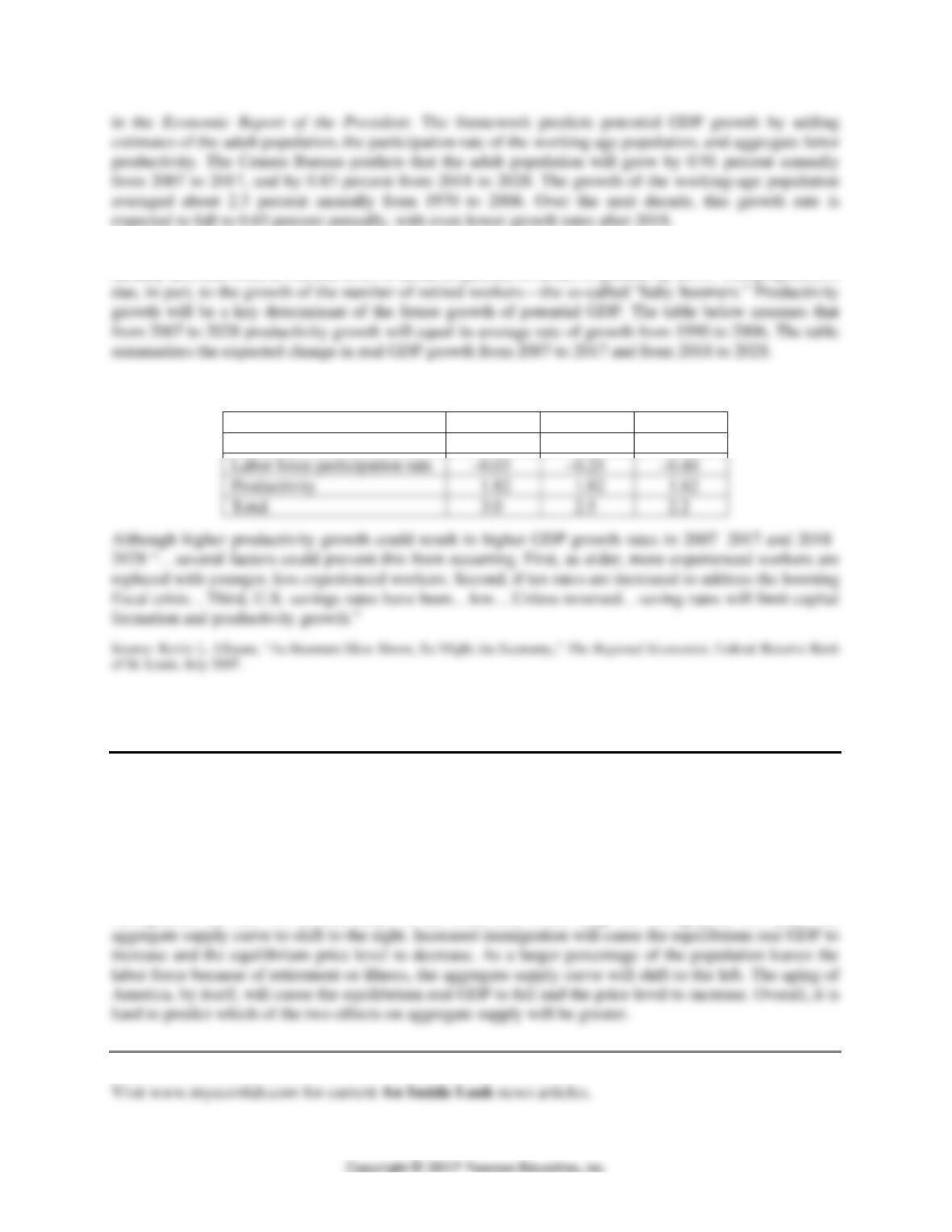
312 CHAPTER 13 | Aggregate Demand and Aggregate Supply Analysis
The trustees of the Social Security Administration estimate that the labor force participation rate will
steadily decrease from its current level of about 66 percent to about 59 percent by 2018. This projection is
Estimated Average Growth Rates for U.S. Potential GDP
Contributions to growth from:
1990–2006
2007–2017
2018–2028
Population
1.25
0.91
0.83
Productivity
1.82
1.82
1.82
Total
Extra Economics in Your Life:
How Will Immigration and an Aging Labor Force Affect You?
Question: Suppose that the friends you made on an international trip are thinking of moving to the
United States. The number of immigrants living in the United States rose 16 percent in recent years,
according to data from the Census Bureau. At the same time, the percentage of the U.S. population over
65 is increasing much faster than the percentage of the population under age 20. How will the increased
immigration and the aging of America affect your standard of living?
Answer: Increased immigration over time leads to a larger supply of labor. Although many believe that
immigration can hurt the United States in the short run, in the long run immigration will cause the
Extra AN INSIDE LOOK News Article to Use in Class