143
CHAPTER 12
TEACHING NOTES
Most of this chapter deals with serial correlation, but it also explicitly considers
heteroskedasticity in time series regressions. The first section allows a review of what
assumptions were needed to obtain both finite sample and asymptotic results. Just as with
heteroskedasticity, serial correlation itself does not invalidate R-squared. In fact, if the data are
stationary and weakly dependent, R-squared and adjusted R-squared consistently estimate the
population R-squared (which is well-defined under stationarity).
Section 12.2 is somewhat untraditional in that it begins with an asymptotic t test for AR(1) serial
correlation (under strict exogeneity of the regressors). It may seem heretical not to give the
Durbin-Watson statistic its usual prominence, but I do believe the DW test is less useful than the
t test. With nonstrictly exogenous regressors I cover only the regression form of Durbin’s test, as
the h statistic is asymptotically equivalent and not always computable.
I do not usually cover Section 12.5 in a first-semester course, but, because some econometrics
packages routinely compute fully robust standard errors, students can be pointed to Section 12.5
if they need to learn something about what the corrections do. I do cover Section 12.5 for a
master’s level course in applied econometrics (after the first-semester course).
SOLUTIONS TO PROBLEMS
12.1 We can reason this from equation (12.4) because the usual OLS standard error is an
estimate of
/x
SST
/x
SST
. When the dependent and independent variables are in level (or log) form,
the AR(1) parameter,
, tends to be positive in time series regression models. Further, the
.
12.2 This statement implies that we are still using OLS to estimate the
j. But we are not using
12.3 (i) Because U.S. presidential elections occur only every four years, it seems reasonable to
think the unobserved shocks – that is, elements in ut – in one election have pretty much
dissipated four years later. This would imply that {ut} is roughly serially uncorrelated.
(ii) The t statistic for H0:
= 0 is −.068/.240 −.28, which is very small. Further, the
12.4 This is false, and a source of confusion in several textbooks. (ARCH is often discussed as a
way in which the errors can be serially correlated.) As we discussed in Example 12.9, the errors
12.5 (i) There is substantial serial correlation in the errors of the equation, and the OLS standard
errors almost certainly underestimate the true standard deviation in
ˆEZ
. This makes the usual
145
12.6 With the strong heteroskedasticity in the errors it is not too surprising that the robust
12.7 (i) The usual Prais-Winsten standard errors will be incorrect because the usual
transformation will not fully eliminate the serial correlation in ut. The regression of the OLS
(ii) Equation (12.32) shows the transformed equation used by the Prais-Winsten method
(without the first time period, which is unimportant for this discussion). If the AR(1) model is
misspecified then the error term in (12.32), et, is still serially correlated. But the Newey-West
(iii) If we drop the homoskedasticity assumption then the et in equation (12.32) exhibit
heteroskedasticity as well as serial correlation. But Newey-West handles both problems at the
SOLUTIONS TO COMPUTER EXERCISES
C12.1 Regressing
ˆt
u
on
1
ˆt
u−
, using the 69 available observations, gives
ˆ
.292 and se(
ˆ
)
.118. The t statistic is about 2.47, and so there is significant evidence of positive AR(1) serial
146
C12.2 (i) After estimating the FDL model by OLS, we obtain the residuals and run the regression
ˆt
u
on
1
ˆt
u−
, using 272 observations. We get
ˆ
.503 and
ˆ
t
9.60, which is very strong
evidence of positive AR(1) correlation.
C12.3 (i) The test for AR(1) serial correlation gives (with 35 observations)
ˆ
–.110, se(
ˆ
)
.175. The t statistic is well below one in absolute value, so there is no evidence of serial
C12.4 (i) After obtaining the residuals
ˆt
u
from equation (11.16) and then estimating (12.48), we
(ii) When we add
21t
return −
to the equation we get
147
(iii) Given our finding in part (ii) we can use WLS with the
ˆt
h
obtained from the quadratic
(iv) To obtain the WLS using an ARCH variance function we first estimate the equation in
C12.5 (i) Using the data only through 1992 gives
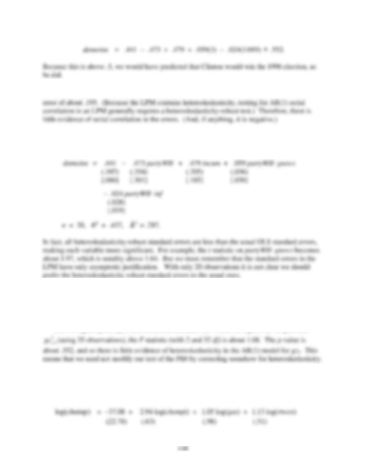
The largest t statistic is on incum, which is estimated to have a large effect on the probability of
winning. But we must be careful here. incum is equal to 1 if a Democratic incumbent is running
and –1 if a Republican incumbent is running. Similarly, partyWH is equal to 1 if a Democrat is
(ii) There are two fitted values less than zero, and two fitted values greater than one.
(iii) Out of the 10 elections with demwins = 1, 8 of these are correctly predicted. Out of the
(v) The regression of
ˆt
u
on
1
ˆt
u−
produces
ˆ
-.164 with heteroskedasticity-robust standard
(vi) The heteroskedasticity-robust standard errors are given in [
] below the usual standard
errors:
C12.6 (i) The regression
ˆt
u
on
1
ˆt
u−
(with 35 observations) gives
ˆ
−.089 and se(
ˆ
)
.178;
there is no evidence of AR(1) serial correlation in this equation, even though it is a static model
in the growth rates.
(ii) We regress gct on gct-1 and obtain the residuals
ˆt
u
. Then, we regress
2
ˆt
u
on gct-1 and
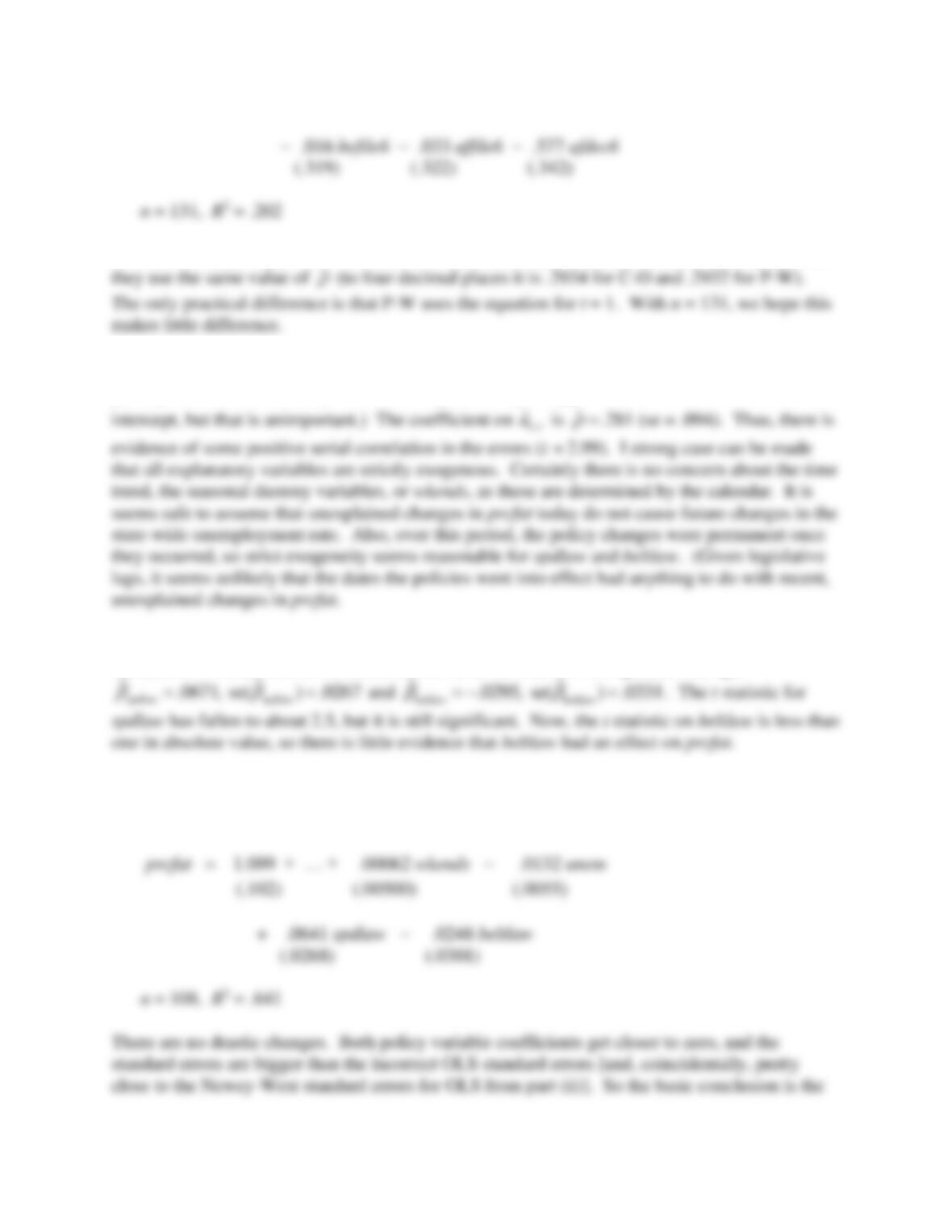
C12.7 (i) The iterated Prais-Winsten estimates are given below. The estimate of
is, to three
decimal places, .293, which is the same as the estimate used in the final iteration of Cochrane-
Orcutt:
149
(ii) Not surprisingly, the C-O and P-W estimates are quite similar. To three decimal places,
C12.8 (i) This is the model that was estimated in part (vi) of Computer Exercise C10.11. After
getting the OLS residuals,
ˆt
u
, we run the regression
1
ˆˆ
on , 2,…,108.
tt
u u t
−=
(Included an
(ii) Remember, we are still estimating the
j by OLS, but we are computing different
standard errors that have some robustness to serial correlation. Using Stata 7.0, I get
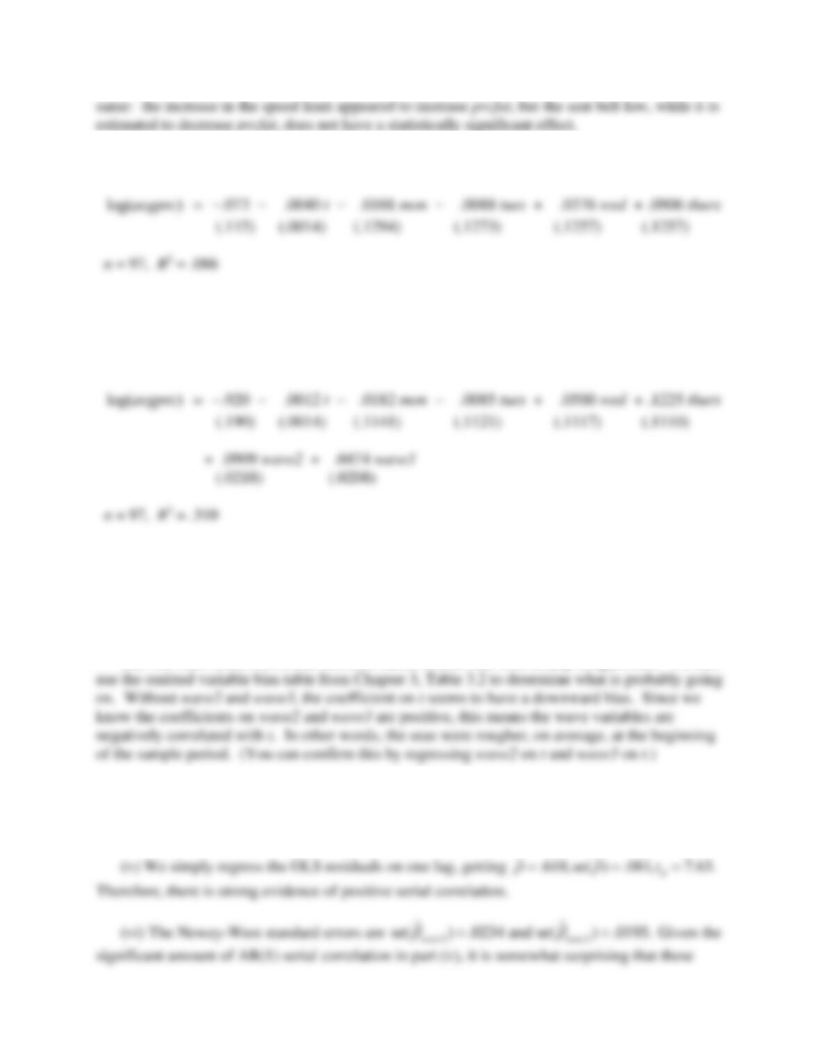
(iii) For brevity, I do not report the time trend and monthly dummies. The final estimate of
is
ˆ.289:
=
150
C12.9 (i) Here are the OLS regression results:
The test for joint significance of the day-of-the-week dummies is F = .23, which gives p-value =
.92. So there is no evidence that the average price of fish varies systematically within a week.
(ii) The equation is
Each of the wave variables is statistically significant, with wave2 being the most important.
Rough seas (as measured by high waves) would reduce the supply of fish (shift the supply curve
back), and this would result in a price increase. One might argue that bad weather reduces the
demand for fish at a market, too, but that would reduce price. If there are demand effects
captured by the wave variables, they are being swamped by the supply effects.
(iii) The time trend coefficient becomes much smaller and statistically insignificant. We can
(iv) The time trend and daily dummies are clearly strictly exogenous, as they are just
functions of time and the calendar. Further, the height of the waves is not influenced by past
unexpected changes in log(avgprc).
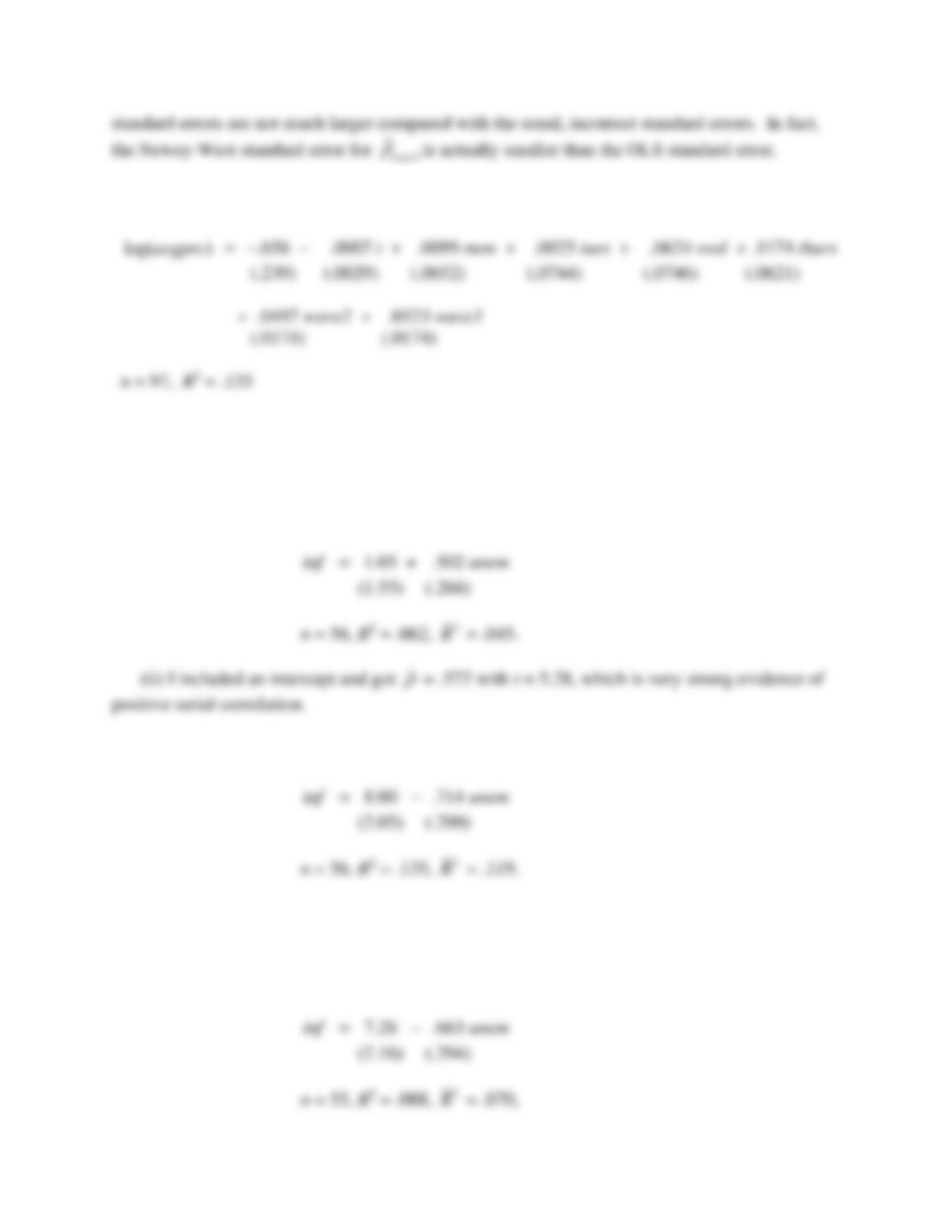
151
(vii) The Prais-Winsten estimates are
The coefficient on wave2 drops by a nontrivial amount, but it still has a t statistic of almost 3.
The coefficient on wave3 drops by a relatively smaller amount, but its t statistic (1.86) is
borderline significant. The final estimate of
is about .687.
C12.10 (i) OLS estimation using all of the data gives
(iii) The iterative Prais-Winsten estimates are
The slope estimate, −.714, is almost identical to that using the data through 1996, −.716.
(Adding more data has reduced the standard error.)
(iv) The iterative C-O estimates are
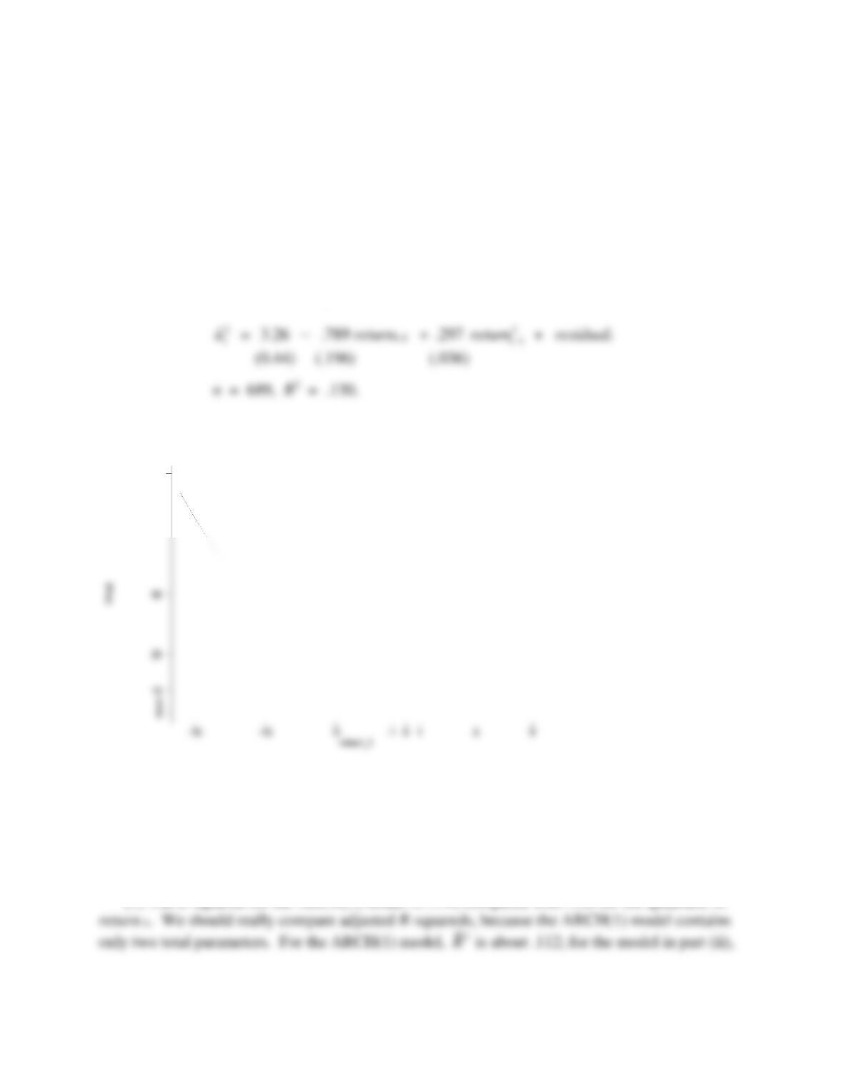
152
and the final estimate of
is .782. The final estimate of
for PW is .789, which is very close to
the C-O estimate. The slope coefficients differ by more than we might expect: −.663 for CO
and −.714 for PW. Using the first observation has a some effect, although the estimates give the
same basic story.
C12.11 (i) The average of
2
ˆi
u
over the sample is 4.44, with the smallest value being .0000074
and the largest being 232.89.
(ii) This is the same as C12.4, part (ii):
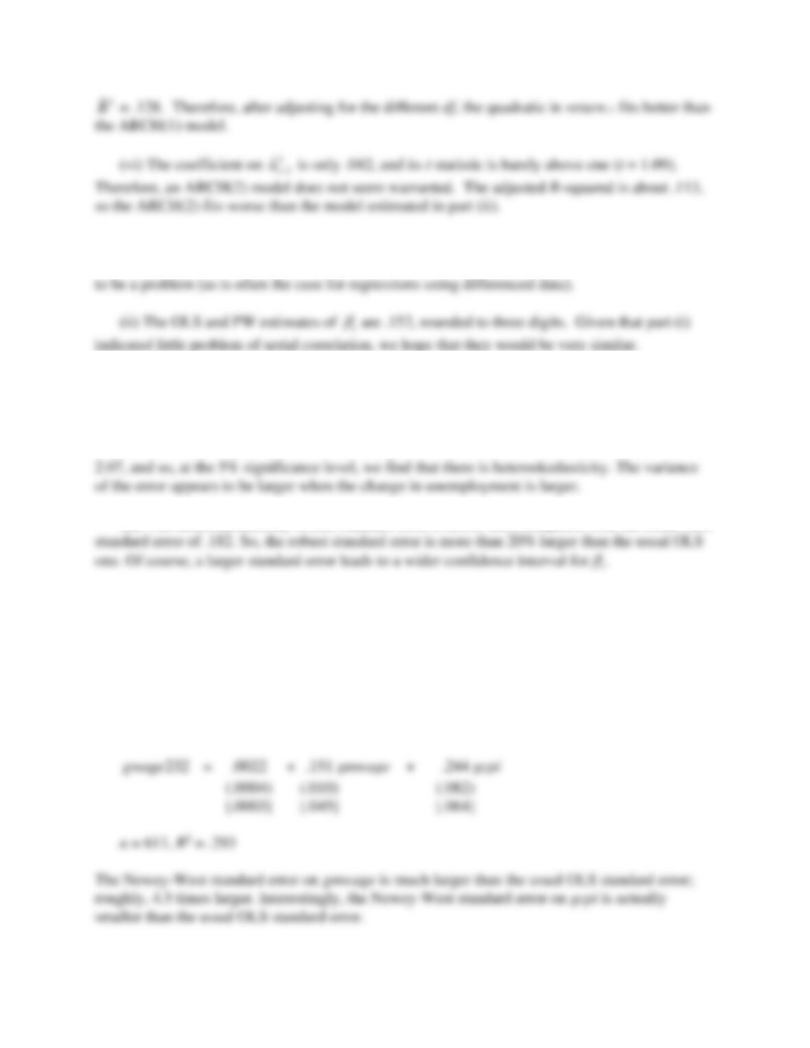
(iii) The graph of the estimated variance function is
The variance is smallest when return-1 is about 1.33, and the variance is then about 2.74.
(iv) No. The graph in part (iii) makes this clear, as does finding that the smallest variance
estimate is 2.74.
(v) The R-squared for the ARCH(1) model is .114, compared with .130 for the quadratic in
100
153
C12.12 (i) The regression for AR(1) serial correlation gives
ˆ
= −.110 with t = −.63. The
estimate of rho is small and statistically insignificant, so AR(1) serial correlation does not appear
C12.13 (i) The regression
ˆt
u
on
1
ˆt
u−
,
t
unem
gives a coefficient on
1
ˆt
u−
of .073 with t = .42.
Therefore, there is very little evidence of first-order serial correlation.
(ii) The simple regression
2
ˆt
u
on
t
unem
gives a slope coefficient of about .452 with t =
(iii) The heteroskedasticity-robust standard error is about .223, compared with the usual OLS
C12.14 (i) The test that maintains strict exogeneity gives
ˆ
= −.097 (t = −2.41), whereas the
regression that includes gmwaget and gcpit gives
ˆ
= −.098 (t = −2.42). Therefore, we find
evidence of some negative serial correlation, and it does not matter which form of the test we
use.
(ii) The estimated equation, with the usual OLS standard errors in () and the twelve-lag
Newey-West standard errors in [], is
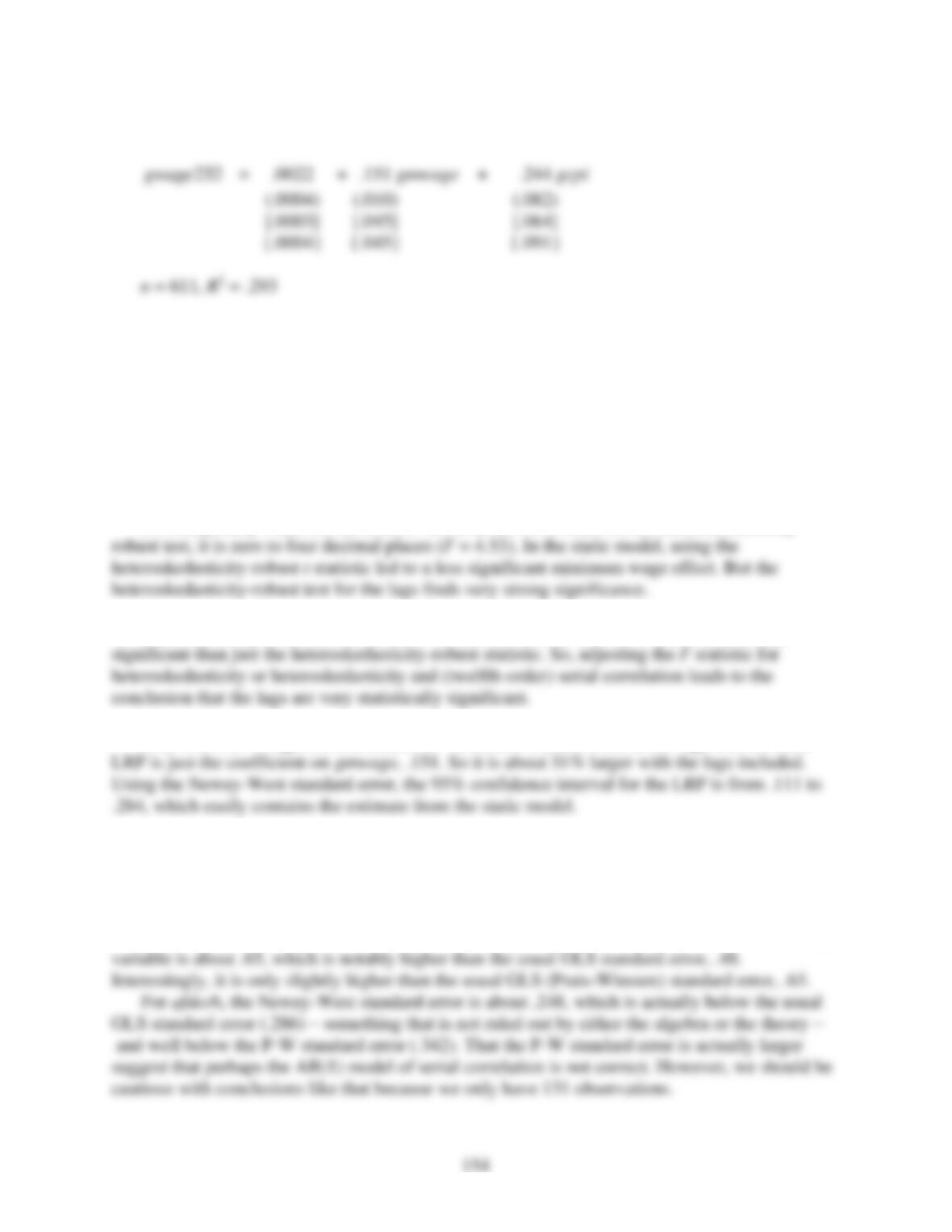
(iii) The equation with heteroskedasticity-robust standard errors in {} is
Certainly for the key variable, gmwage, heteroskedasticity is where all the action is. Adjusting
the standard error for serial correlation in addition to heteroskedasticity – which is what Newey-
West does – makes no difference. Probably because of the negative serial correlation, adjusting
the standard error on gcpi actually reduces it. Heteroskedasticity does not have a major effect on
the gcpi standard error.
(iv) The Breusch-Pagan test gives F = 233.8, which implies a p-value of essentially zero.
There is very strong evidence of heteroskedasticity.
(v) Oddly, the p-value for the usual F test is about .058, while for the heteroskedasticity-
(vi) The Newey-West version of the F statistic is 7.79, which is even more statistically
(vii) With the 12 lags, the estimated LRP is about .198, and without the lags the estimated
C12.15 (i) If there is in fact AR(1) serial correlation in the errors, then the OLS standard errors
are invalid. With positive AR(1) serial correlation, the OLS estimates usually have a downward
bias: they are too small, on average.
(ii) Using the command newey in Stata, with a lag of four, the standard error for the lchempi
155
(iii) Interestingly, as we go from g = 4 to g = 12, the standard error on lchempi increases to
.741 while that on afdec6 decreases rather sharply, to .195. In any case, we can conclude that