286 CHAPTER 12 | Aggregate Expenditure and Output in the Short Run
Appendix
The Algebra of Macroeconomic Equilibrium (pages 812–813)
Learning Objective: Apply the algebra of macroeconomic equilibrium.
Graphs and tables are alternative means to illustrate the aggregate expenditure model of short-run real
GDP. Graphs help us understand economic change qualitatively. We make it easier to make quantitative
estimates when we write down an economic model using equations. When economists forecast future
movements in GDP, they often rely on econometric models. An econometric model is an economic model
written in the form of equations, where each equation has been statistically estimated. The following
equations are based on the example from Table 12.3.
1. C = 1,000 + 0.65Y Consumption function
2. I = 1,500 Planned investment function
This equation can be solved for Y to find equilibrium GDP:
Y = 10,000.
To make this result more general, we can replace particular values with general values represented by
letters:
1.
()C C MPC Y
=+
Consumption function
The letters with bars over them represent fixed, or autonomous, values.
Solving for equilibrium Y:
CHAPTER 12 | Aggregate Expenditure and Output in the Short Run 287
Solutions to End-of-Chapter Exercises
12.1
The Aggregate Expenditure Model
Learning Objective: Understand how macroeconomic equilibrium is determined in the
aggregate expenditure model.
Review Questions
1.1 The key idea of the aggregate expenditure model is that in any particular year the level of real
GDP is determined mainly by the level of aggregate expenditure.
Problems and Applications
1.4 a. Consumption
b. Government purchases
1.5 Because the computer chips Intel sells to Dell are intermediate goods they would not be included
in spending on goods and services or aggregate expenditure. Aggregate expenditure would
increase if Dell sells the computers that include the computer chips as components.
1.6 a. If companies are drawing down their inventories, aggregate expenditure would be greater
than GDP.
288 CHAPTER 12 | Aggregate Expenditure and Output in the Short Run
1.9 It does matter that Japanese firms didn’t expect the decrease in demand to be as great as it was
because it resulted in an unplanned increase in inventories. Because the decline in demand was
12.2
Determining the Level of Aggregate Expenditure in the Economy
Learning Objective: Discuss the determinants of the four components of aggregate
expenditure and define marginal propensity to consume and marginal propensity
to save.
Review Questions
2.1 In the aggregate expenditure model, real GDP changes only when aggregate expenditure changes,
so it is crucial to understand the factors that change each of the four categories of aggregate
expenditure.
2.2 The five main determinants of consumption spending are current disposable income, household
wealth, expected future income, the price level, and the interest rate. The most important
determinant is current disposable income. A rise in stock prices or housing prices would increase
household wealth, which would increase consumption spending.
Problems and Applications
2.6 a. This development would increase the forecast demand for appliances because the rise in
consumer confidence that income growth will be increasing would likely increase consumption
spending.
CHAPTER 12 | Aggregate Expenditure and Output in the Short Run 289
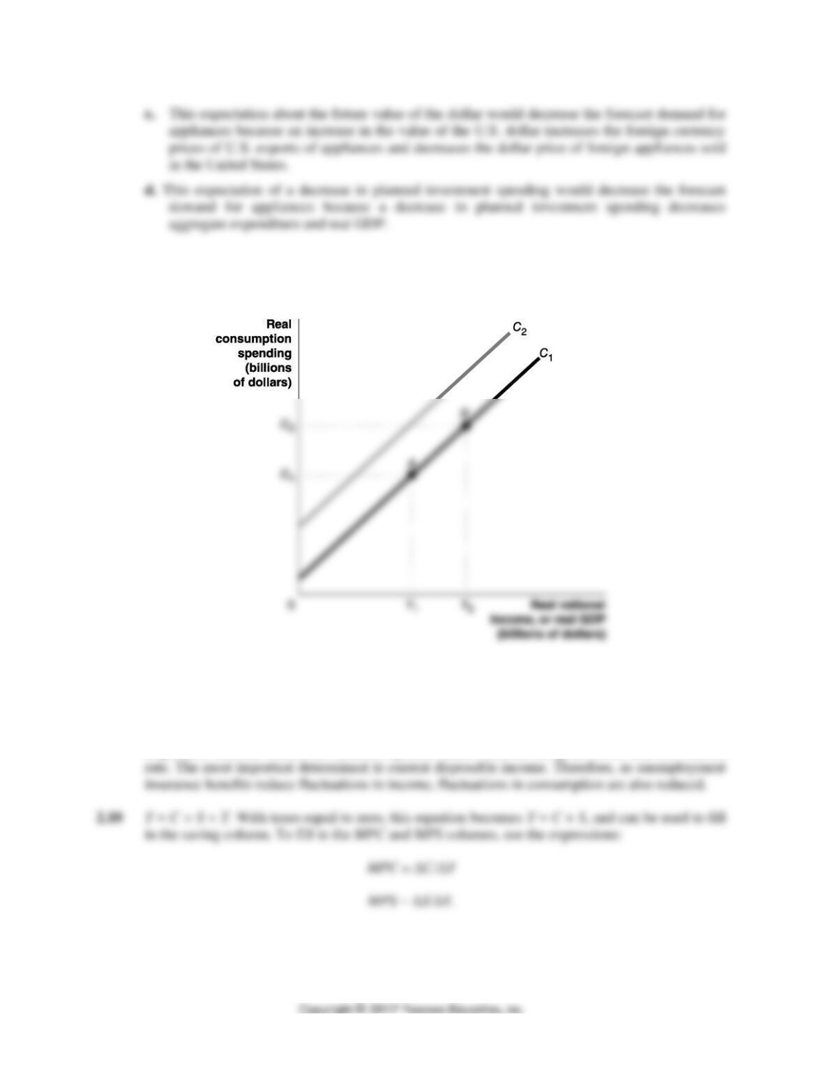
2.7 In the graph of the consumption function below, an increase in income from Y1 to Y2 increases
consumption spending along the consumption function C1 (A to B). An increase in expected
future income or household wealth shifts the consumption function upward, from C1 to C2.
2.8 The student’s reasoning is incorrect because he or she has confused investment in the economic
sense—which involves purchasing machinery, factories, and houses—with financial investment
or saving.
2.9 Consumption will fluctuate less. The five main determinants of consumption spending are current
disposable income, household wealth, expected future income, the price level, and the interest
290 CHAPTER 12 | Aggregate Expenditure and Output in the Short Run
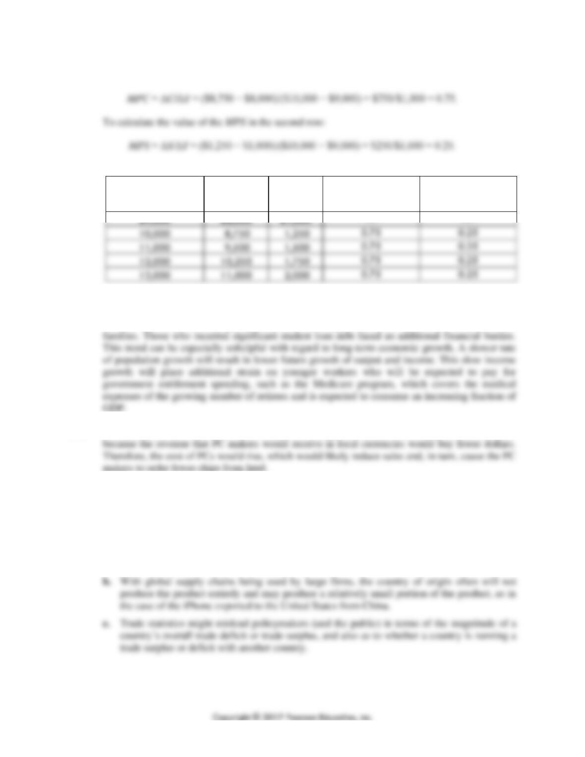
For example, to calculate the value of the MPC in the second row:
National Income and
Real GDP
(Y)
Consumption
(C)
Saving
(S)
Marginal Propensity
to Consume
(MPC)
Marginal Propensity
to Save
(MPS)
—
—
2.11 There are a number of reasons why young adults delay getting married and having children. One
reason is financial. The severity of the 2007-2009 recession and the subsequent sluggish recovery
limited the ability of many young adults to find employment and to afford to start their own
2.12 An increase in the value of the dollar relative to foreign currencies would likely hurt Intel’s sales
2.13 d. iPhones are assembled in China using components produced by many firms located in several
different countries. The BEA’s use of the “country of origin” concept to measure imports
overstates the value of imports from China and other countries.
2.14 a. Conventional trade statistics treat imported goods as produced entirely within the country of
origin. This approach dates to a time when most products were produced entirely within one
country.
CHAPTER 12 | Aggregate Expenditure and Output in the Short Run 291
12.3
Graphing Macroeconomic Equilibrium
Learning Objective: Use a 45-line diagram to illustrate macroeconomic equilibrium.
Review Questions
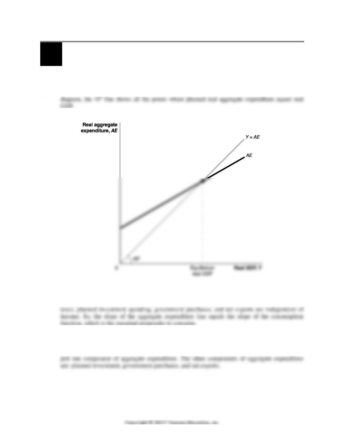
3.1 The 45° line represents all the points that are equal distances from both axes. In the 45°–line
3.2
3.3 The slope of the aggregate expenditure line is the change in aggregate expenditure based on a
change in real GDP (ΔAE/ΔReal GDP). The simple aggregate expenditure model assumes that
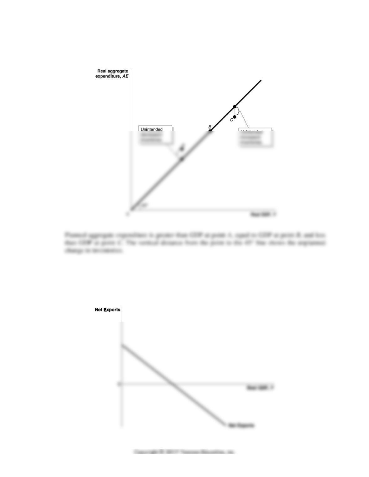
3.4 Firms will decrease production until they sell the unintended inventories.
3.5 Aggregate expenditure represents the total spending in the economy. Consumption spending is
292 CHAPTER 12 | Aggregate Expenditure and Output in the Short Run
Problems and Applications
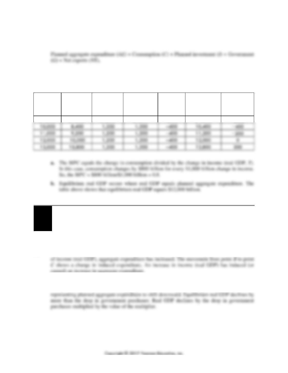
3.6
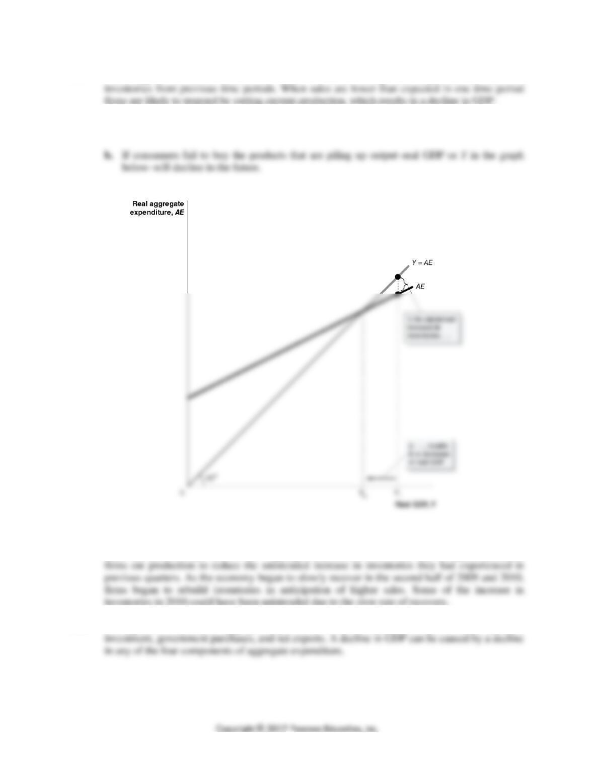
3.7 Net exports equal the value of exports minus the value of imports. Net exports is graphed as a
downward-sloping line because although increases in U.S. real GDP will not directly affect U.S.
exports, these increases will cause imports to increase and net exports to decline, holding other
factors constant. As real GDP increases, net exports eventually become negative, which they have
typically been for the United States in recent years.
CHAPTER 12 | Aggregate Expenditure and Output in the Short Run 293
3.8 “Shedding of unwanted inventories” refers to firms selling their unplanned increases in
3.9 a. Business inventories must have increased during this period since “products are piling up in
warehouses.”
3.10 Inventories climbed during 2007 as the economy slowed down and moved into recession. In 2008
and 2009, with the significant drop in aggregate expenditure in the economy during the recession,
3.11 The argument is incorrect. Aggregate expenditure includes not just consumption but also planned
294 CHAPTER 12 | Aggregate Expenditure and Output in the Short Run
3.12 Calculate the missing values in the last two columns of the table by using two equations:
and
Unplanned change in inventories = Real GDP (Y) − Planned aggregate expenditure (AE).
Real GDP
(Y)
Consumption
(C)
Planned
Investment
(I)
Government
Purchases
(G)
Net Exports
(NX)
Planned
Aggregate
Expenditure
(AE)
Unplanned
Change in
Inventories
$ 9,000
$ 7,600
$1,200
$1,200
–$400
$ 9,600
−$600
8,400
9,200
10,000
12.4
The Multiplier Effect
Learning Objective: Describe the multiplier effect and use the multiplier formula to
calculate changes in equilibrium GDP.
Review Questions
4.1 The movement from point A to point B shows a change in autonomous expenditure. At each level
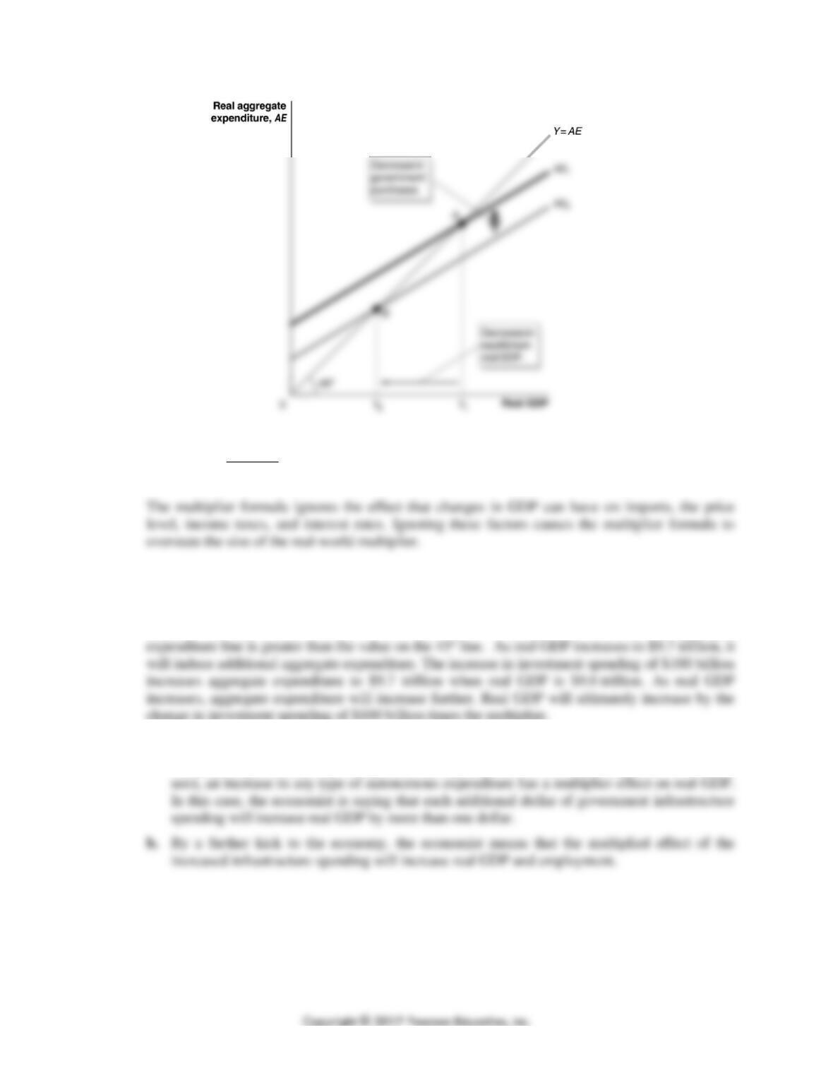
4.2 The multiplier effect is the process by which a change in autonomous expenditure leads to a
change in real GDP. In the following graph, the decrease in government purchases causes the line
CHAPTER 12 | Aggregate Expenditure and Output in the Short Run 295
4.3 Multiplier =
1
1MPC−
.
Problems and Applications
4.4 No, because when real GDP equals $9.7 trillion, aggregate expenditure is greater than $9.7
trillion. We know this because at real GDP of $9.7 trillion, the value on the aggregate
4.5 a. Government spending on infrastructure, such as bridges and highways, is in the expenditure
category of government spending rather than private investment spending. But as we have
296 CHAPTER 12 | Aggregate Expenditure and Output in the Short Run
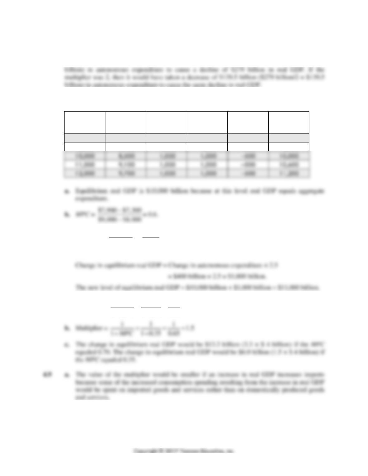
4.6 From 1929 to 1933, real GDP declined $279 billion from $1,057 billion to $778 billion. If the
multiplier was 4, then it would have taken a decrease of $69.75 billion ($279 billion/4 = $69.75
4.7 We can answer this question by adding a column in the table for aggregate expenditure.
Real GDP
(Y)
Consumption
(C)
Planned
Investment
(I)
Government
Purchases
(G)
Net Exports
(NX)
Aggregate
Expenditure
(AE)
$8,000
$7,300
$1,000
$1,000
–$500
$8,800
9,000
7,900
1,000
1,000
–500
9,400
10,000
8,500
1,000
1,000
–500
10,000
11,000
9,100
1,000
1,000
–500
10,600
12,000
9,700
1,000
1,000
–500
11,200
c. Multiplier =
1
1MPC
=
−
12.5
1 0.6
=
−
.
So,
4.8 a. Multiplier =
1 1 1 3.3
1 1 0.70 0.30MPC
= = =
−−
CHAPTER 12 | Aggregate Expenditure and Output in the Short Run 297
b. The value of the multiplier would be smaller if an increase in real GDP increases interest
rates. An increase in interest rates decreases planned investment spending, consumption
spending on durable goods, and net exports (as a result of the appreciation in the value of the
U.S. dollar).
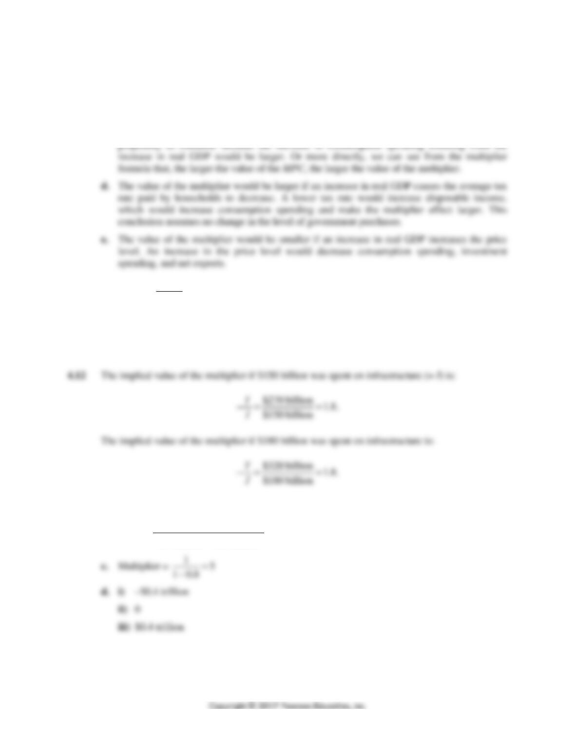
c. The value of the multiplier would be larger if an increase in real GDP increases the marginal
4.10 Multiplier =
15
1 0.8
=
−
Change in equilibrium GDP = −$75 billion × 5 = −$375 billion.
4.11 A larger multiplier would be likely to lead to longer and more severe recessions because it would
magnify the effect on the economy of changes in autonomous expenditures.
4.13 a. $12 trillion
b. MPC =
$13.6 trillion –$12 trillion
$14trillion –$12 trillion
= 0.8
298 CHAPTER 12 | Aggregate Expenditure and Output in the Short Run
12.5
The Aggregate Demand Curve
Learning Objective: Understand the relationship between the aggregate demand curve
and aggregate expenditure.
Review Questions
5.1 Aggregate expenditure is the total amount of spending in the economy, and aggregate demand is
the relationship between the price level and the level of planned aggregate expenditure.
Problems and Applications
5.4 An upward-sloping aggregate expenditure line reflects the positive relationship between real GDP
and aggregate expenditure, while a downward-sloping aggregate demand curve reflects the
inverse relationship between the price level and the level of planned aggregate expenditure.
5.5 You should disagree with the statement that the aggregate demand curve slopes downward
Real-Time Data Exercises
D12.1 a. Download data from FRED on real exports from 1990 to the present.
b. Real exports of goods and services decreased from $1,790.0 billion in the second quarter of
CHAPTER 12 | Aggregate Expenditure and Output in the Short Run 299
Solutions to Chapter 12 Appendix
Review Questions
12A.1 AE = (
C
+
I
+
G
+
NX
) + MPC (Y)
The intercept would be (
C
+
I
+
G
+
NX
) and the slope would be equal to the value of the MPC.
12A.2 Y = 1,500 + 0.75Y + 1,250 + 1,250 + (−250); Y = 3,750 + 0.75Y;
12A.3 AE = $3,750 + 0.75Y
For GDP of $16,000, aggregate expenditure = $3,750 + 0.75($16,000) = $15,750.