Economics Chapter 12 Recap of the Aggregate Demand and Supply

Chapter 12

The Aggregate Demand and Supply Model

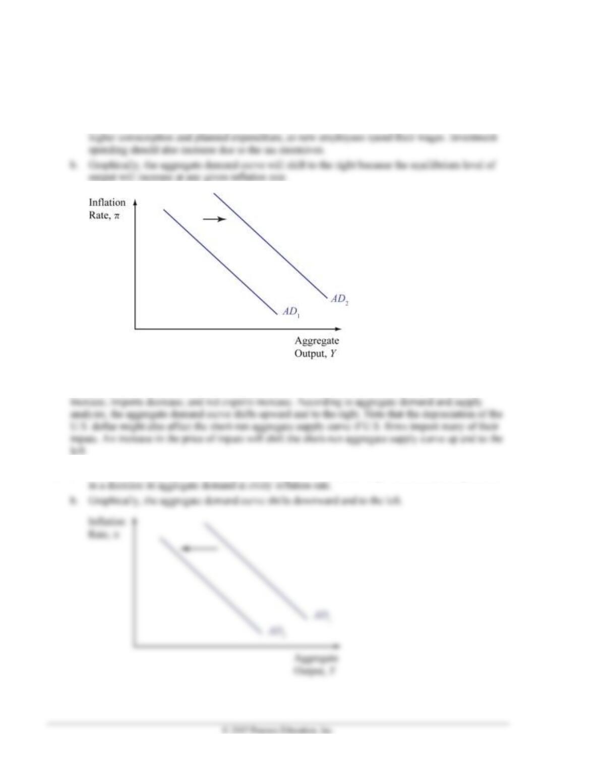
◼ Chapter Outline, Overview, and Teaching Tips

Chapter Outline

Recap of the Aggregate Demand and Supply Curves

The Aggregate Demand Curve

Factors That Shift the Aggregate Demand Curve

Equilibrium in Aggregate Demand and Supply Analysis

Short-Run Equilibrium

Changes in Equilibrium: Aggregate Demand Shocks

Application: The Volcker Disinflation, 1980–1986

Application: Negative Demand Shocks, 2001–2004

Changes in Equilibrium: Aggregate Supply (Price) Shocks

Temporary Supply Shocks

AD/AS Analysis of Foreign Business Cycle Episodes

Application: The United Kingdom and the 2007–2009 Financial Crisis

Application: China and the 2007–2009 Financial Crisis

Chapter 12 The Aggregate Demand and Supply Model 121

Chapter Overview and Teaching Tips

Now students are ready for the payoff from their work in understanding all the building blocks in the

previous three chapters. The resulting aggregate demand/aggregate supply model differs from that in many

other textbooks because it is inherently dynamic and emphasizes the interaction of inflation and economic

activity. In contrast to older AD/AS frameworks which have the price level on the vertical axis, the

dynamic AD/AS approach in this textbook has inflation on the vertical axis.

The chapter starts with a recap of the aggregate demand and supply curve. All this material repeats the

analysis in the previous chapters, but I think it is very important to go over this again in class because it

puts all the analysis together at one time. Also, recaps like this are a good way of getting students to really

understand the material. It is again helpful in class to make use of the teaching device of the summary

tables in the text, 12.1 and 12.2, which summarize what factors cause the aggregate demand and supply

curves to shift. Listing changes in the variables that shift the AD and AS curves and then asking students to

fill in the tables by saying which way the curves will shift and the reasons behind the shift will give them

the practice they need to master the model.

The rest of the chapter shows how inflation and equilibrium output changes as a result of either aggregate

demand shocks or aggregate supply (price) shocks. To drive home the analysis and also show students

how useful the AD/AS model is, the chapter goes through a large number of applications. The first two,

“The Volcker Disinflation, 1980–1986” and “Negative Demand Shocks, 2001–2004,” demonstrate how

122 Mishkin • Macroeconomics: Policy and Practice, Second Edition

The chapter has three online appendices on the companion Website, www.pearsonhighered.com/mishkin.

The first formally demonstrates a point made in Chapter 10 that the Taylor principle is necessary for

inflation stability and, thus ,provides the rationale for why a central bank has to raise the real interest rate

◼ Answers to End of Chapter Review Questions and Problems

Answers to Review Questions

Recap of Aggregate Demand and Supply Curves

1. A rise in inflation causes the real interest rate to rise. This reduces planned expenditures and lowers

the level of output necessary for goods market equilibrium. The opposite occurs if inflation falls.

2. The following changes shift the aggregate demand curve to the right: monetary policy easing,

3. Shifts in the short-run aggregate supply curve result from changes in expected inflation, price shocks,

and persistent output gaps. None of these factors shift the long-run aggregate supply curve because

Equilibrium in Aggregate Demand and Supply Analysis

4. Short-run equilibrium requires that the quantity of aggregate output demanded equals the quantity of

output supplied. This occurs where the aggregate demand curve and the short-run aggregate supply

5. When output exceeds potential output, unemployment is below the natural rate, and labor market

tightness causes wages to rise more rapidly. As the Phillips curve suggests, this causes firms to raise

their prices more rapidly and, thus, increases the inflation rate. As a result, expected inflation will be

Chapter 12 The Aggregate Demand and Supply Model 123

Changes in Equilibrium: Aggregate Demand Shocks

6. Demand shocks are exogenous changes that cause the aggregate demand curve to shift. These shocks

7. A positive demand shock moves the aggregate demand curve to the right and causes both inflation

and output to increase. Because this increases output relative to potential output and expands the

Changes in Equilibrium: Aggregate Supply (Price) Shocks

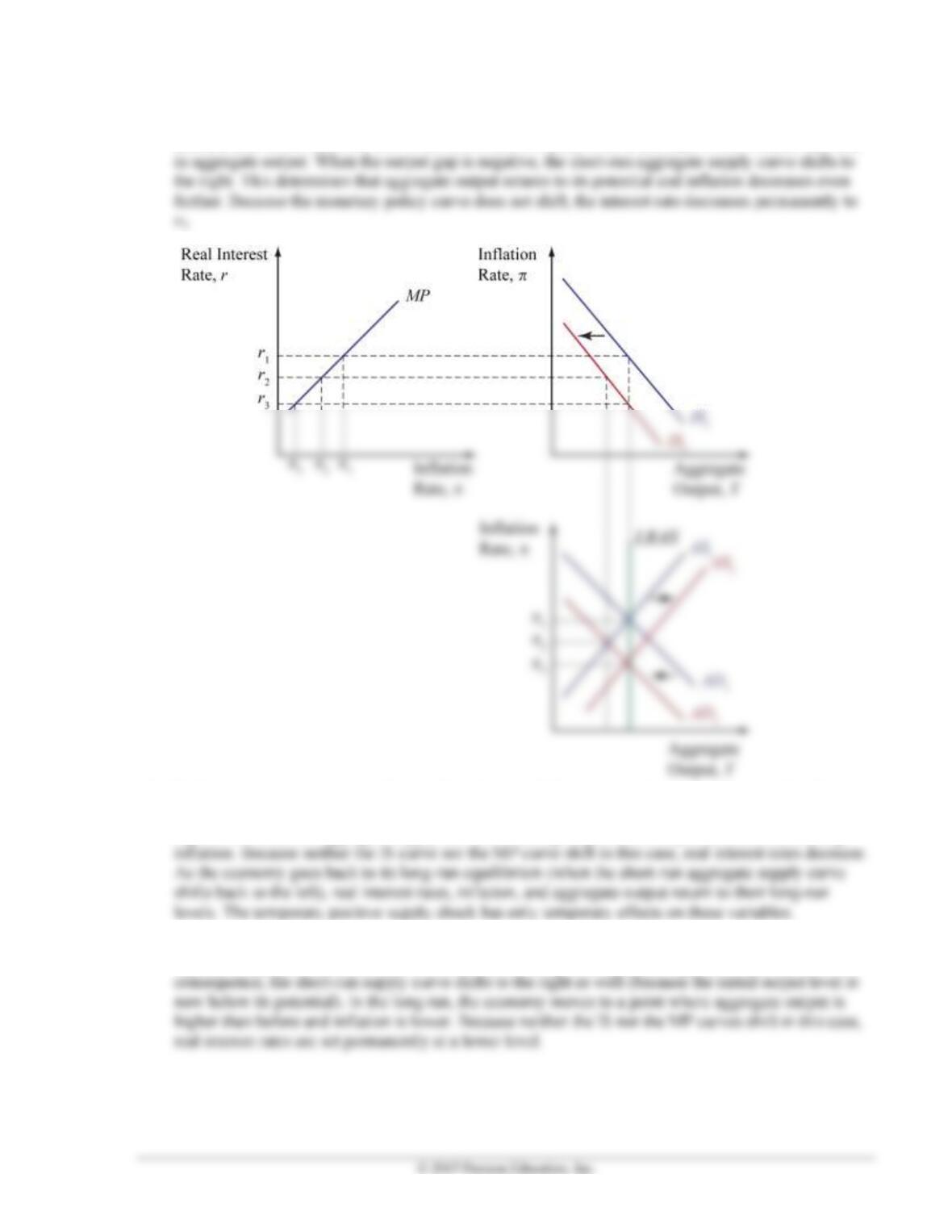
8. Supply shocks are another term for the price shocks that cause shifts of the short-run Phillips curve

and, therefore, of the short-run aggregate supply curve. Positive supply shocks lower inflation and

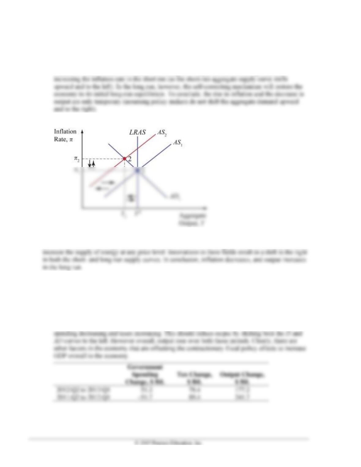
9. The temporary negative supply shock does not affect potential output or the long-run aggregate

supply curve but shifts the short-run aggregate supply curve up and to the left. This initially raises the

inflation rate and causes short-run equilibrium output to fall below potential output. With actual

10. A permanent negative supply shock, unlike a temporary one, reduces potential output and shifts the

long-run aggregate supply curve to the left. Inflation begins to rise, and output falls. Although output

has fallen, potential output also has fallen, the lower output is above the new potential output, and

124 Mishkin • Macroeconomics: Policy and Practice, Second Edition

Answers to Problems

Recap of the Aggregate Demand and Supply Curves

1. a. In general, these proposals will reduce the tax burden on small businesses and encourage

businesses to hire more employees and to increase investment. More employment will result in

2. The statement is correct. A depreciation of the U.S. dollar makes U.S. exports cheaper for foreign

consumers at the same time it makes imports into the U.S. more expensive. As a result, exports

3. a. According to aggregate demand and supply analysis, a decrease in government spending results

Chapter 12 The Aggregate Demand and Supply Model 125

4. The decrease in oil prices made production possible at lower costs by decreasing the price of energy,

transportation, and a number of raw materials. It therefore lessened pressure for firms to raise prices,

Changes in Equilibrium: Aggregate Demand Shocks

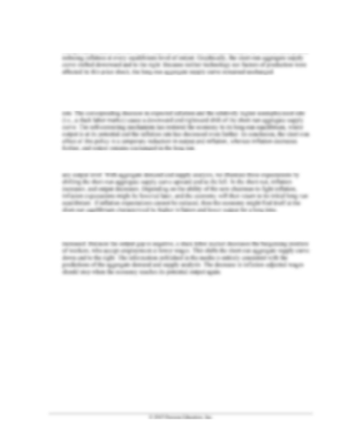
5. The decrease in government spending will result in a decrease in aggregate output at every inflation

rate and, therefore, will shift the aggregate demand curve downward and to the left in the short run.

The economy will be at a short-run equilibrium with output below its potential and a lower inflation

6. The appointment of a Fed chairman who has no interest in fighting inflation will most likely result in

an increase in expected inflation. Both firms and workers will expect inflation rates to be higher at

7. The decline in real (i.e., inflation-adjusted) wages reflects the operation of the self-correcting

mechanism. Due to the combination of the negative supply shock (increase in oil prices) and the

decrease in aggregate demand (from the global financial crisis), output decreased, and unemployment

126 Mishkin • Macroeconomics: Policy and Practice, Second Edition

Changes in Equilibrium: Aggregate Supply (Price) Shocks

8. a. The destruction of crops will negatively affect the supply of food, increasing its price. A decrease

in U.S. oil refinery capacity reduces the supply of gas and makes transportation and energy more

expensive. These events will translate into a negative supply shock, decreasing output and

b. See graph:

9. Technological change affects the long-run aggregate supply curve. More fuel efficient cars result in a

decrease in the demand for gas at the same time that innovations in energy production make it possible to

◼ Answers to Data Analysis Problems

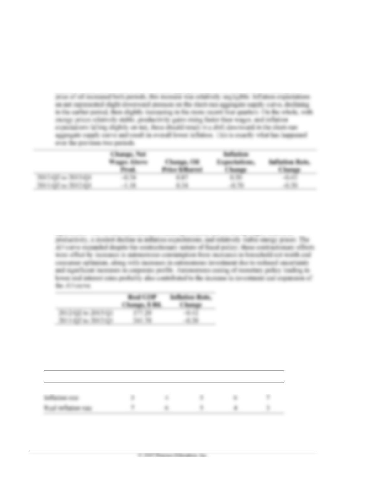
1. a. See summary table below.

b. See summary table below.

c. No, this is not consistent with what would be expected for tax and spending changes. During both

four-quarter periods, a contractionary fiscal policy change took place with both government

Chapter 12 The Aggregate Demand and Supply Model 127

2. a. See summary table below.

b. See summary table below.

c. Yes, the data from part (b) are consistent with what would be expected to explain part (a).

Household net worth increased over both periods, as did consumer sentiment. This should have

3. a. See summary table below.

b. See summary table below.

c. Yes, the data from part (b) are consistent with what would be expected to explain part (a).

Increases in corporate profits, and improvements (negative change) in economic uncertainty

128 Mishkin • Macroeconomics: Policy and Practice, Second Edition

4. a. See summary table below.

b. See summary table below.

c. Yes, the data from part (b) do seem to be consistent with what would be expected to explain part

(a). The change in net wages above productivity was negative for both periods, meaning that

productivity of workers rose faster than wages over those periods, which would put downward

pressure on inflation and shift the short-run aggregate supply curve downward. Although the

5. a. See table below.

b. Over the period from 2011:Q2 to 2013:Q1, on the whole real GDP increased, and inflation fell by

a fair amount. This is consistent with the AS curve shifting down more than the AD curve

expands outward, resulting in a net effect of higher output and lower inflation in a new

equilibrium. The AS curve shifted downward significantly due to falling wages relative to

◼ Answers to Review Questions and Problems in Web Appendix,

“The Taylor Principle and Inflation Stability”

1.

Period 1

Period 2

Period 3

Period 4

Period 5

Nominal interest rate

10

Inflation rate

6

7

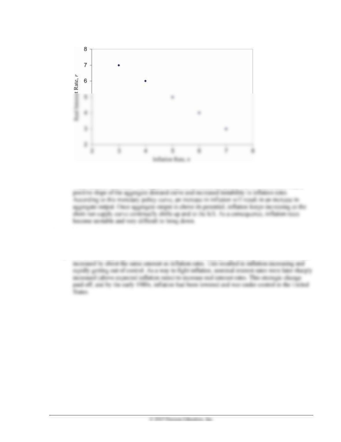
Chapter 12 The Aggregate Demand and Supply Model 129

a.

b. According to this monetary policy curve, monetary policy authorities do not increase nominal

interest rates more than the inflation rate increases, and as a result real interest rates decrease

when inflation increases. The negative slope of the monetary policy curve is associated with a

2. a. If nominal interest rates change by the same amount as inflation, real interest rates remain

unchanged (according to the Fisher equation). A plot of inflation rates on the horizontal axis and

real interest rates on the vertical axis yields a flat monetary policy curve in this case.

b. For some time, policy makers followed the same monetary policy rule and nominal interest rates

130 Mishkin • Macroeconomics: Policy and Practice, Second Edition

◼ Answers to Review Questions and Problems in Web Appendix,

“The Effects of Macroeconomic Shocks on Asset Prices”

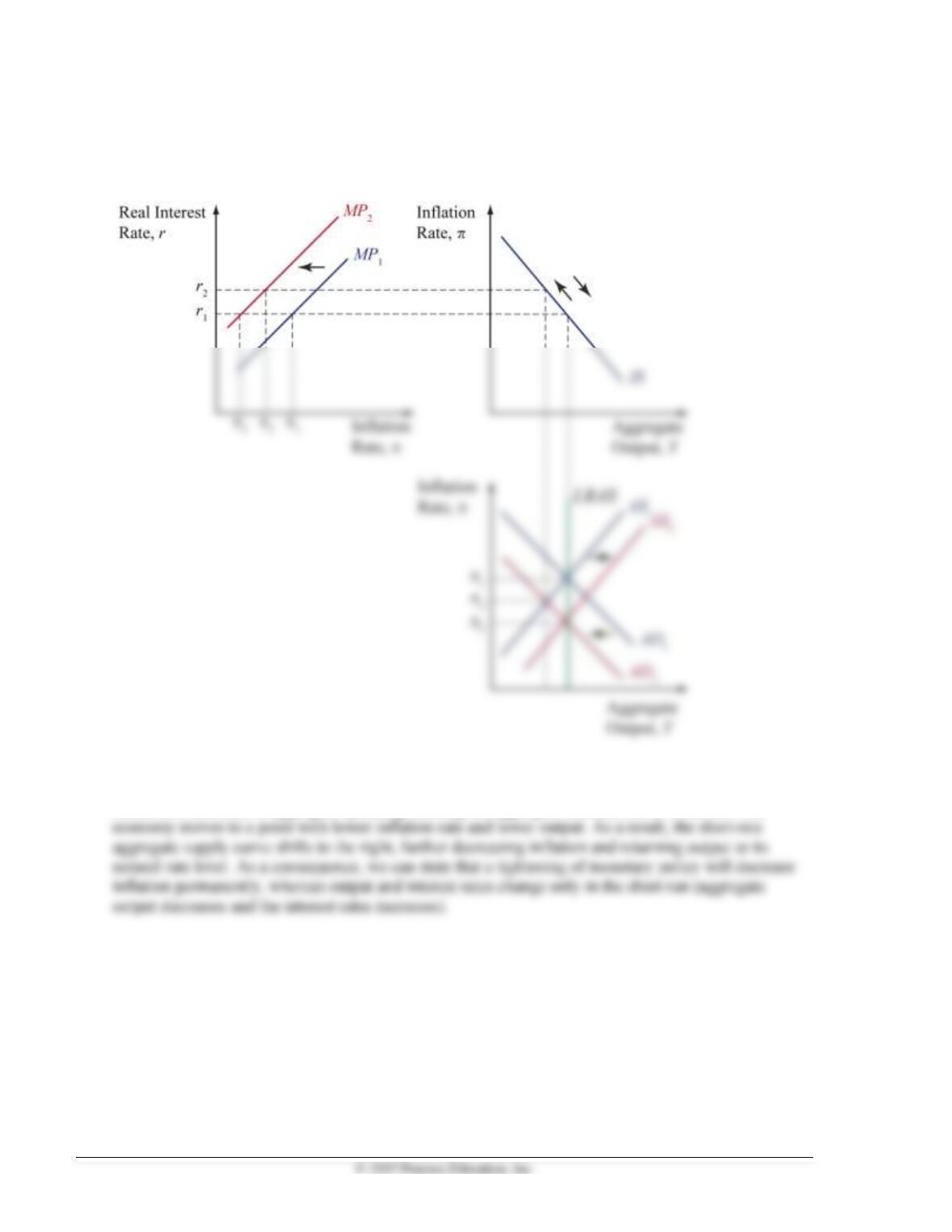
1.

As seen in the graph, a tightening of monetary policy engineered by the Fed will shift the monetary

policy curve up, increasing real interest rates at every inflation rate. An increase in real interest rates

results in a decrease in aggregate spending, shifting the aggregate demand curve to the left. The

Chapter 12 The Aggregate Demand and Supply Model 131

2. As seen in the graph, a decrease in net exports decreases aggregate demand and shifts the aggregate

demand and IS curves to the left. In the short run, this determines a decrease in the inflation rate and

3. In this context, a rainy season that results in increased electricity production can be considered a

temporary positive supply shock (i.e., a decrease in the price of energy). This results in a shift to the

right of the short-run aggregate supply curve, increasing output above its potential and decreasing

4. This technological advance can be interpreted as a permanent positive supply shock. This is

represented graphically by a shift to the right on the long-run aggregate supply curve. As a

132 Mishkin • Macroeconomics: Policy and Practice, Second Edition

5. a. A monetary policy tightening results in higher interest rates and lower output, decreasing the

denominator and increasing the numerator in Equation A2-1. This results in an unambiguous

decrease in stock prices.

◼ Data Sources, Related Articles, and Discussion Questions

A. For Information About Application: The Volcker Disinflation, 1980–1986

Data Sources

Bureau of Labor Statistics: http://www.bls.gov/cps/. For unemployment rate data, click on the “10 years of

Discussion Questions

Using Figure 12.4, explain why the unemployment rate decreased from 9.7 percent in 1982 to 7.0 percent

in 1986. (Hint: Consider the transition from point 2 to point 3 in the graph.) Can we say that Volcker’s

efforts were successful?

Answer: After the economy finds itself in point 2, the output gap is negative, therefore pushing real wages in

B. For Information About Application: Negative Demand Shocks, 2001–2004

Data Source

events that contributed to the decrease in aggregate demand mentioned in the text). You can get data for

unemployment and inflation using the links provided in the previous application and changing the data

range to 2000–2004.

Chapter 12 The Aggregate Demand and Supply Model 133

of the Enron scandal to other countries.

Discussion Question

In the aftermath of the September 11 attack, the Federal Reserve announced that it would fulfill its

function as lender of last resort to restore confidence in the U.S. financial system. Throughout the year, the

Fed closely followed the developments in stock markets and lowered interest rates during 2001. Do you

agree with the Fed’s actions during these years?

Answer: The Fed’s actions in the aftermath of the terrorist attacks in 2001 were effective in restoring

C. For Information About Application: Negative Supply Shocks, 1973–1975

and 1978–1980

Data Source

Federal Reserve Bank of St. Louis database (FRED):

Using the aggregate demand and supply model, explain what happened to the unemployment and inflation

rate between 1975 and 1978 (the in-between negative shocks period).

Answer: According to the aggregate demand and supply model, after the 1973 negative supply temporary

D. For Information About Application: Positive Supply Shocks, 1995–1999

Data Source

numbers&series_id=PRS85006092. Here you can find data about labor productivity in the nonfarm

business sector. You can change the data range to 1990 to 2000 to observe the positive rate of change in

this series during the 1995–1999 periods.

134 Mishkin • Macroeconomics: Policy and Practice, Second Edition

Discussion Question

Based on your knowledge of the production function and drivers of growth discussed in Chapter 7, how

can you explain the effects of the “new economy” on the production function?

Answer: The “new economy” entered the production function by increasing total factor productivity (i.e.,

E. For Information About Application: Negative Supply and Demand Shocks

and the 2007–2009 Financial Crisis

Data Source

Bureau of Labor Statistics: http://www.bls.gov/cps/. For unemployment rate data, click on the “10 years of

historical data” icon (the green dinosaur) and select 2006 to 2010 to get data shown in panel (b) in Figure

Discussion Question

The Federal Reserve was criticized for supporting the U.S. financial system during the 2007–2009 crisis.

Using the aggregate demand and supply model, explain what would have happened if the Fed refused to

help some major participants in the U.S. financial system.

Answer: The financial crisis entered its more virulent stage in 2008, when some high profile firms in the

F. For Information About Application: The United Kingdom and the 2007–2009

Financial Crisis

Data Source

Federal Reserve Bank of St. Louis database (FRED):

Chapter 12 The Aggregate Demand and Supply Model 135

Discussion Question

During 2008, the British government borrowed heavily and used part of these funds to recapitalize British

banks hit by the financial crisis. Using the aggregate demand and supply model, explain the effects of

supporting the financial system on unemployment and inflation.

Answer: Actions taken by the British authorities, in conjunction with the Bank of England, had similar

G. For Information About Application: China and the 2007–2009 Financial

Crisis

Data Source

International Monetary Fund database:

Discussion Question

China was not affected as the United Kingdom was during the 2007–2009 financial crisis; tt was affected

only when other countries experienced a recession that resulted in a decrease in Chinese exports. Explain

where this difference comes from.

Answer: The Chinese economy (and its financial system in particular) is still heavily controlled by the