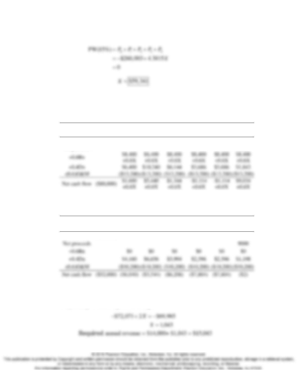
• The break–even rental:
12.14 Let X denotes the additional annual revenue (above $14,000) for model A that
is required to break even.
• Generalized cash flow for model A:
Cash flow
elements
End of Year
0
1
2
3
4
5
6
Investment
($80,000)
Net proceeds
12,000
$6,400
$3,686
$1,843
PW(20%) $72,071 2
AX=−+
• Generalized cash flow for model B:
Cash flow
elements
End of Year
0
1
2
3
4
5
6
Investment
($52,000)
($10,200)
($10,200)
($52,000)
($6,040)
($3,544)
($7,804)
PW(20%) $69,985
B
= −
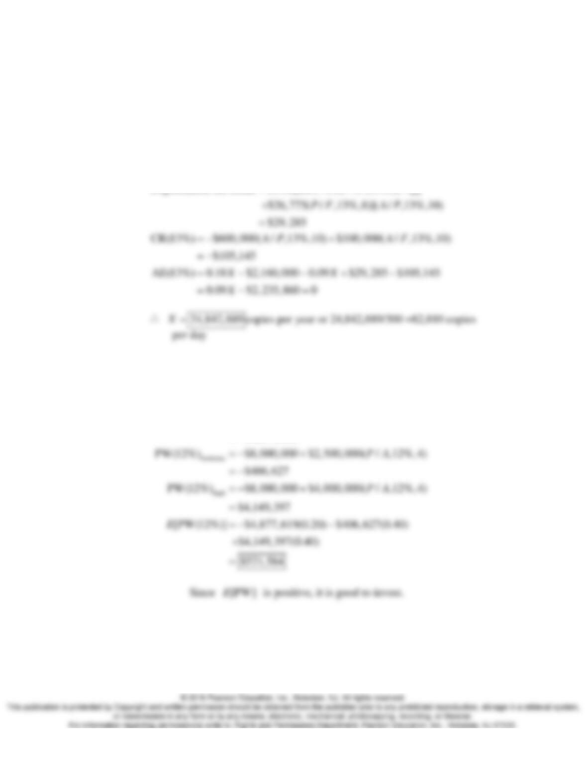
• By letting
AB
PW(20%) = PW(20%)
12.15
Let X denote the number of copies to break-even.
• A/T annual revenue
(0.6)[$0.05 $0.25]X= +
0.18X=
• A/T O&M cost
(0.60)[$300,000(12) $0.15 ]X=−+
$2,160,000 0.09X=−−
Depreciation tax credit (0.40)[$85, 714( / ,13%,1)
P F
= +
Probabilistic Analysis
12.16
light
PW(12%) $8, 000,000 $1,300,000( / ,12%,3)
$4,877, 619
PA
=−+
= −
12.17
(a)
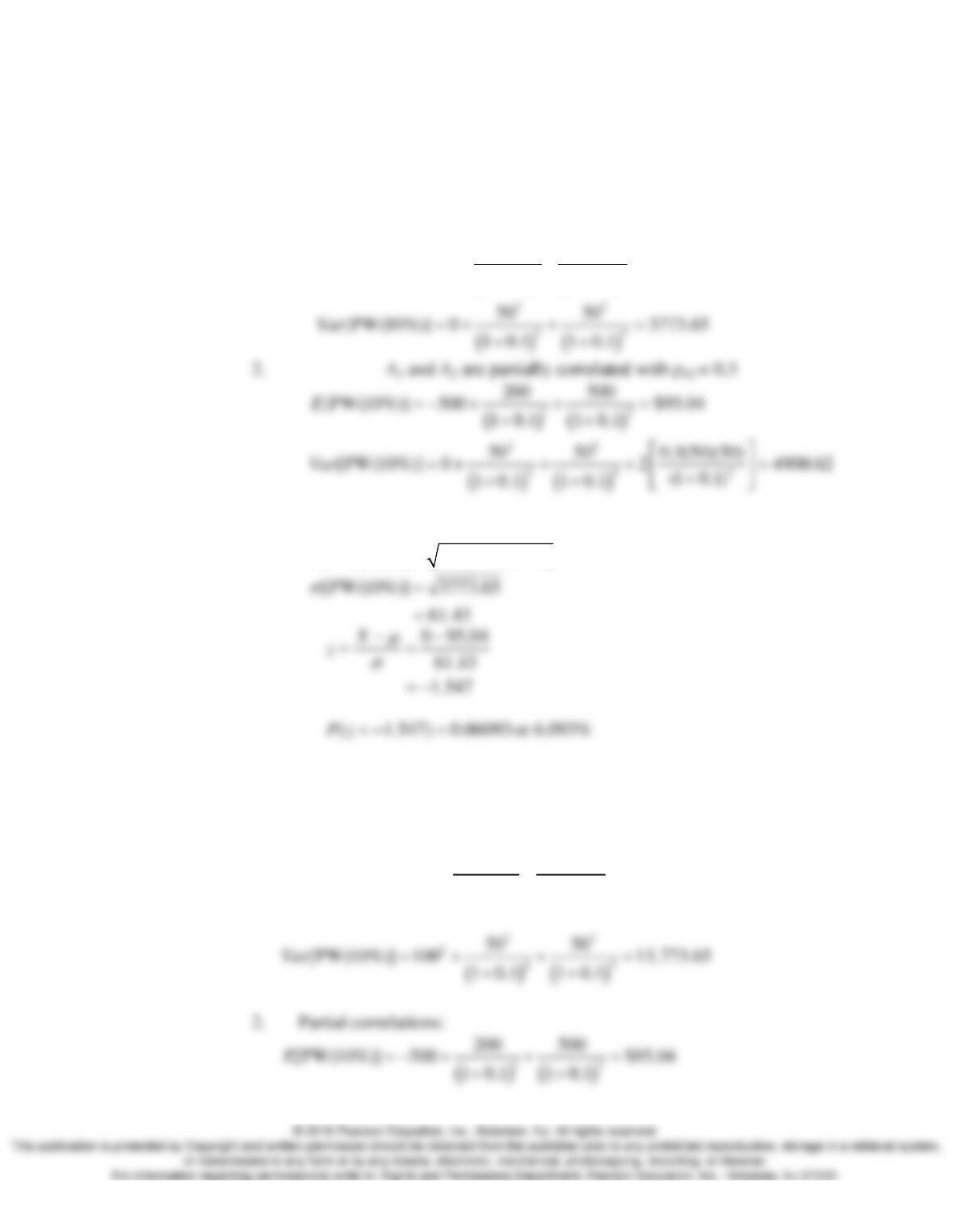
1. A1 and A2 are mutually independent
( ) ( )
12
200 500
[PW(10%)] 500 $95.04
1 0.1 1 0.1
E=−+ + =
++
(b)
[PW(10%)] [PW(10%)]Var
σ
=
12.18
(a)
1. Mutually independent:
( ) ( )
12
200 500
[PW(10%)] 500 $95.04
1 0.1 1 0.1
E=−+ + =
++
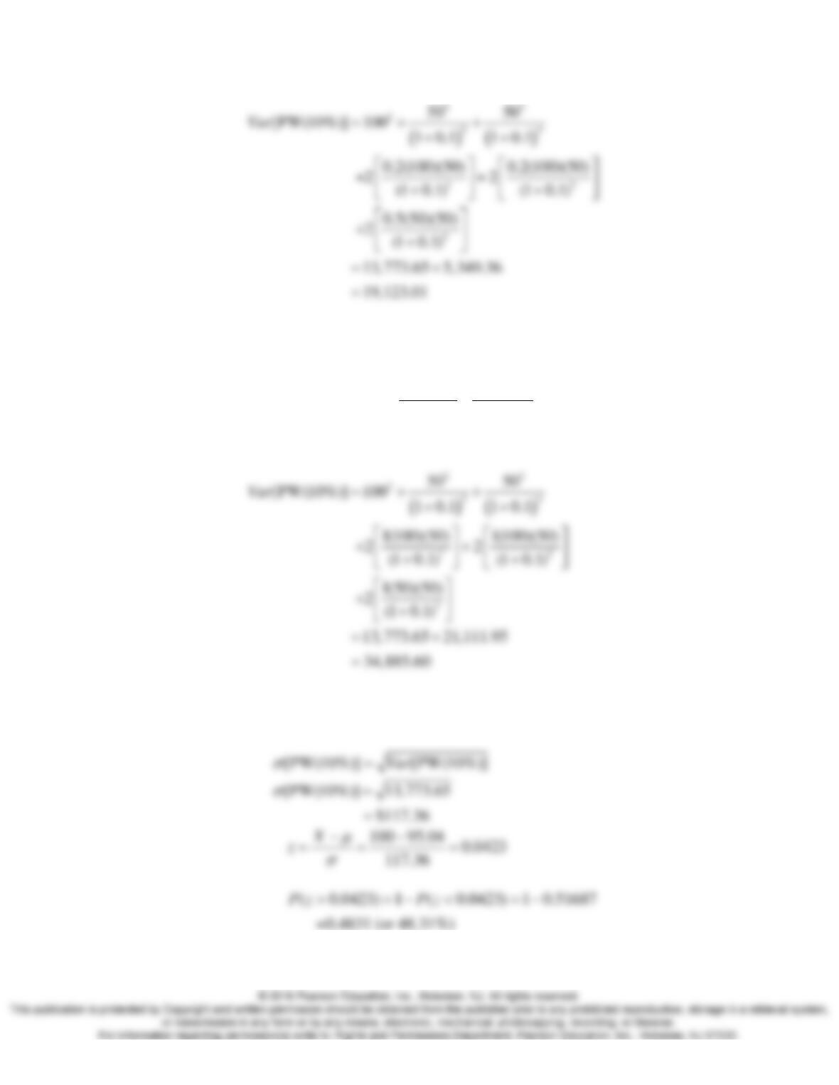
3. Perfect positive correlations:
( ) ( )
12
200 500
[PW(10%)] 500 $95.04
1 0.1 1 0.1
E=−+ + =
++
(b)
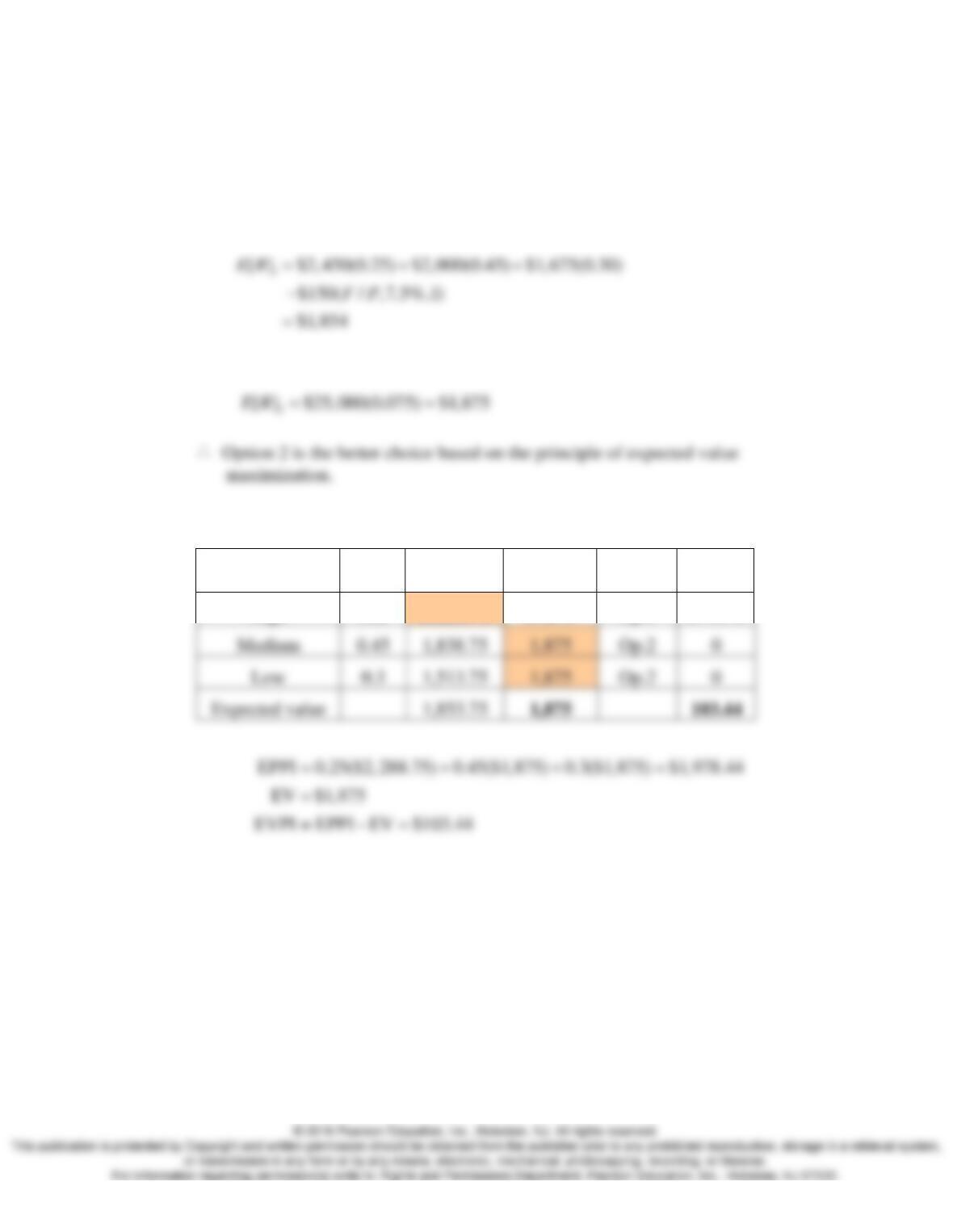
12.19 Expected value criterion:
(a)
• Option 1:
• Option 2:
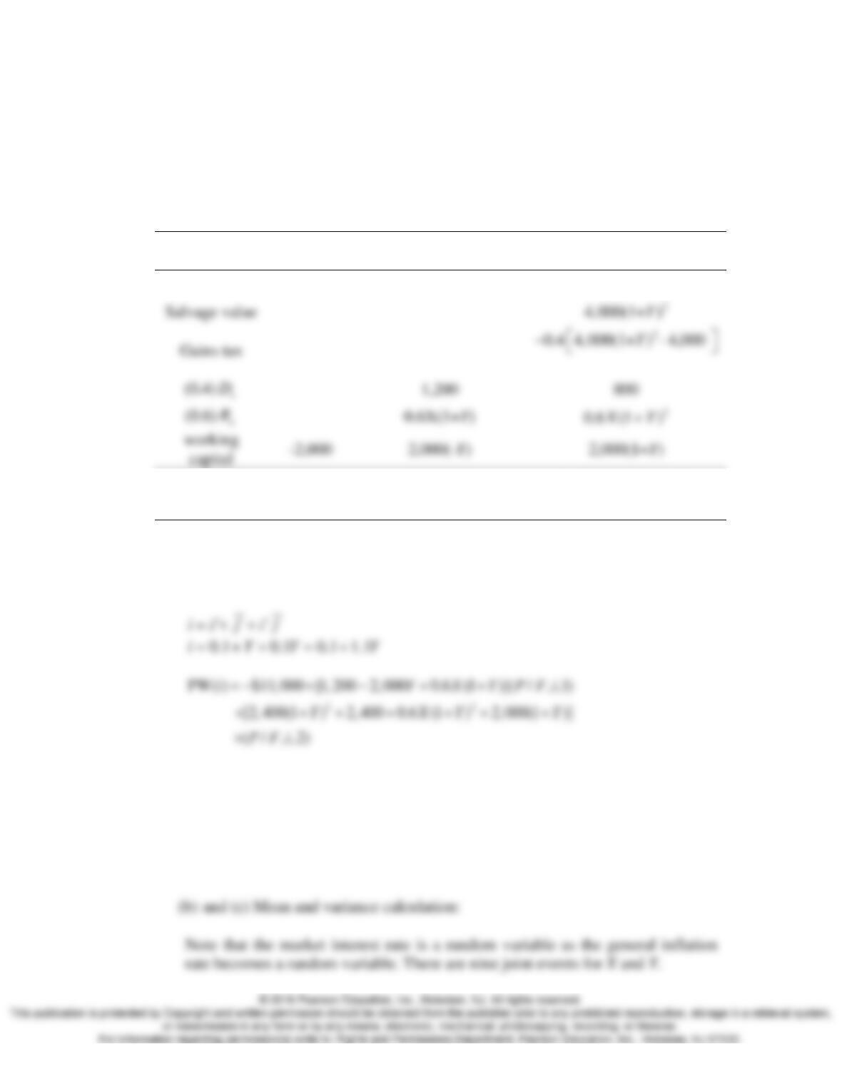
(b)
Potential return
Prob.
Op.1
Op.2
Optimal
choice
Opp.
Loss
High
0.25
$2,288.75
$1,875
Op.1
$413.75
0.45
1,838.75
Op.2
0.3
1,513.75
Op.2
1,853.75
12.20
Let X denote the annual revenue in constant dollars and Y be the general inflation.
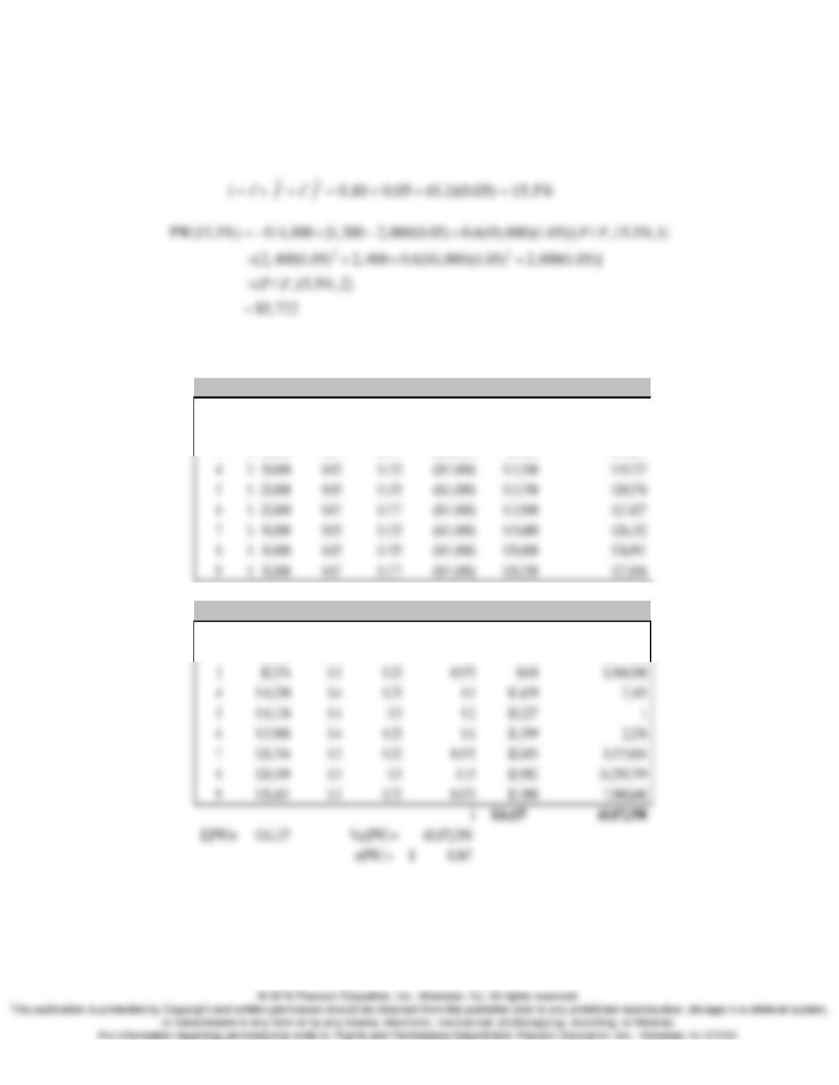
(a) NPW as functions of X and Y:
Cash elements
End of Period
0
1
2
Investment -$9,000
Net cash
flow(Actual) -$11,000 1,200-2,000Y
+0.6X(1+Y)
2,400
(1+Y)2
+2,400
+0.6X
2
(1+ )Y
+2,000(1+Y)
Net cash
flow(Constant) -$11,000
-1
1
1, 200(1+ )
2,000 (1+ ) 0.6
Y
YY X
−
−+
2
-1
2,400 2, 400(1+ )
0.6 2,000(1+ )
Y
XY
−
+
++
or
-1 1
2 -1
PW(10%) $11,000 [1, 200(1 ) 2,000 (1 ) 0.6 ]( / ,10%,1)
[2, 400 2, 400(1 ) 0.6 2, 000(1 ) ]( / ,10%, 2)
Y Y Y X PF
Y X Y PF
−
−
=− + +− + +
+ + ++ + +
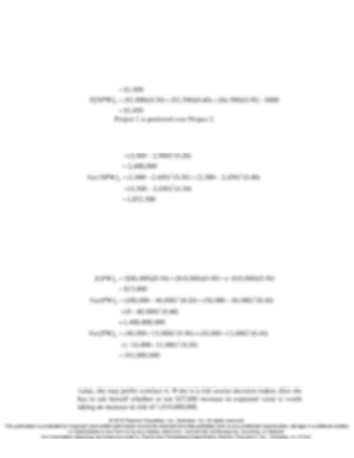
For example of event No.2, the joint event where X
10,000=
and Y
0.05=
, we
calculate the market interest rate and then evaluate the PW function with this
market interest rate.
You repeat the process for the remaining joint events.
Event No. X Y i A0 A1 A2
1 10,000$ 0.03 0.133 ($11,000) $7,320 $13,372
2 10,000$ 0.05 0.155 ($11,000) $7,400 $13,761
3 10,000$ 0.07 0.177 ($11,000) $7,480 $14,157
Event No. PW(i%) P(x) P(y) P(x,y)
PW(i%)*P(x,y) (PW(i%)-E[PW])^2*P(x,y)
1 $5,877 0.3 0.25 0.075 $441 7,895,197
2 $5,722 0.3 0.5 0.15 $858 16,270,806
Comparing Risky Projects
12.21
(a)
1
[NPW] ($2,000)(0.20) ($3,000)(0.60) ($3,500)(0.20) $1,000
E
=++−
(b)
22
1
[NPW] (2,000 2,900) (0.20) (3,000 2,900) (0.60)
=− +−
Var
∴ No project dominance.
12.22
(a) Mean and variance calculations:
1
[PW] ($100,000)(0.20) ($50,000)(0.40) (0)(0.40)
$40,000
E
= ++
=
It is not a clear case, because
1 2
E E>
but also
1 2
Var Var>
.
If she makes decision solely based on the principle of maximization of expected
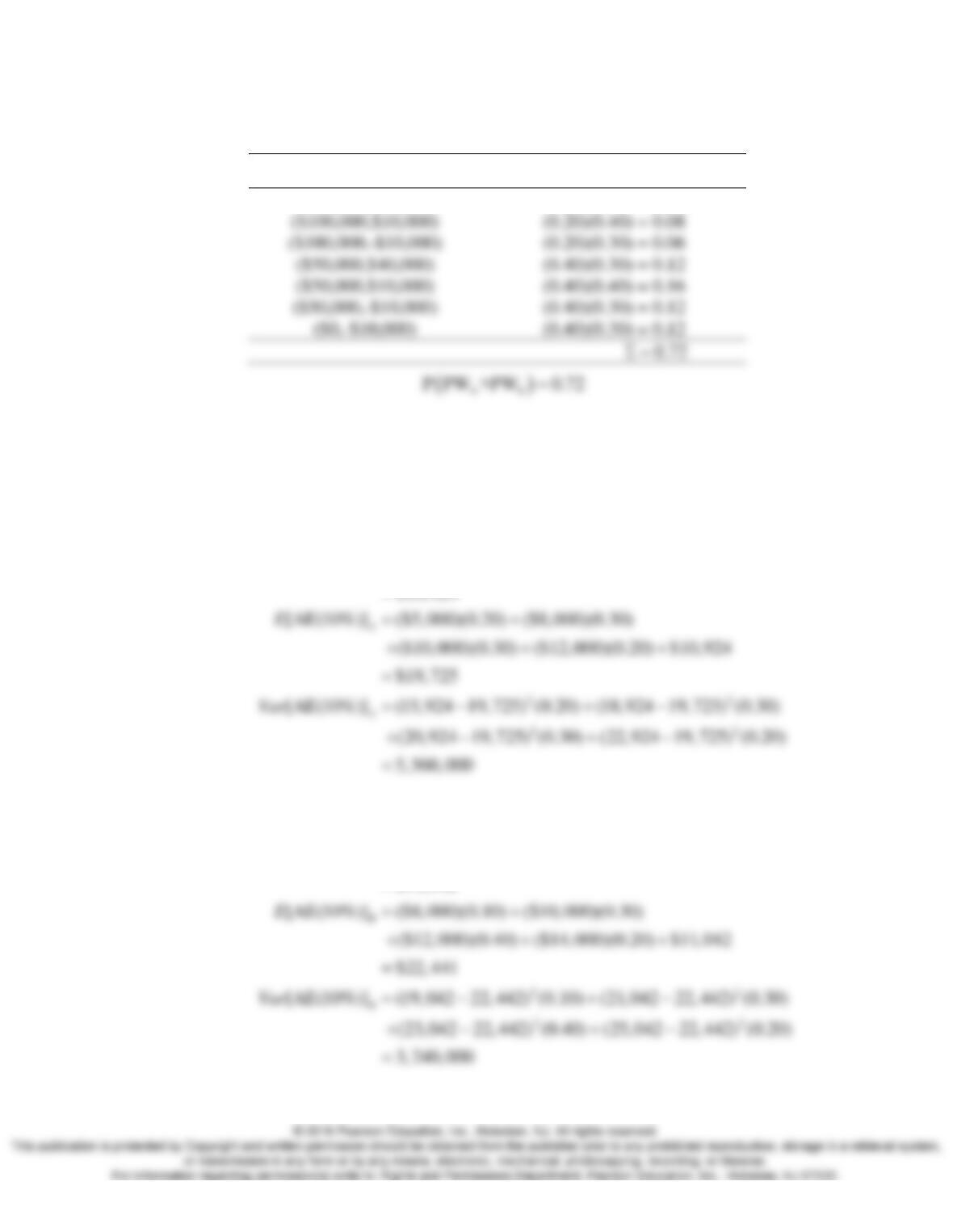
(b) Assuming that both contracts are statistically independent from each other,
12.23
(a)
• Machine A:
CR(10%) ($60,000 $22,000)( / ,10%,6) (0.10)($22,000)
$10,924
A
AP
=−+
=
• Machine B:
CR(10%) $35,000( / ,10%, 4)
$11, 042
B
AP
=
=
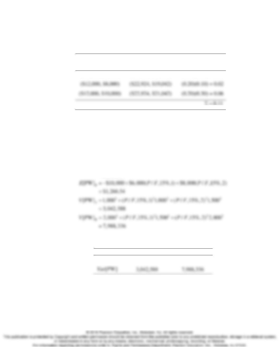
Joint event
AB
(PW >PW )
Joint Probability
($100,000,$40,000)
(0.20)(0.30) = 0.06
($100,000,$10,000)
(0.20)(0.40) = 0.08
(0.20)(0.30) = 0.06
(0.40)(0.30) = 0.12
(0.40)(0.40) = 0.16
(0.40)(0.30) = 0.12
(b)
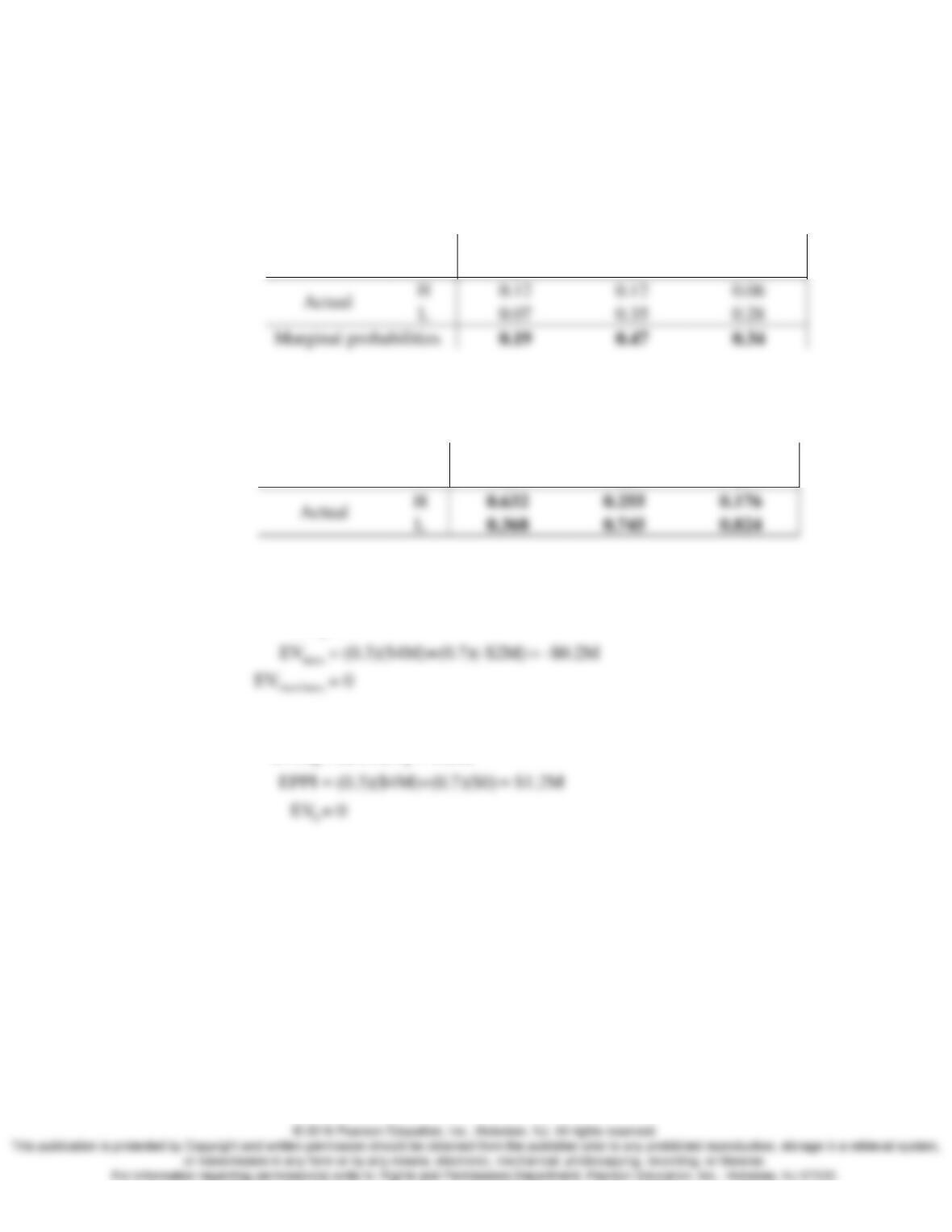
Prob[ (10%) (10%) ] :
A B
AE AE>
Joint event
AB
(O&M ,O&M )
AB
(AE >AE )
Joint
Probability
($10,000, $8,000)
($20,924, $19,042)
(0.30)(0.10) = 0.03
0.11Σ =
12.24
(a) Mean and variance calculation (Note: For a random variable Y, which can be
expressed as a linear function of another random variable X (say, Y =
aX
,
where
a
is a constant) the variance of Y can be calculated as a function of
variance of X,
2
[ ] [ ]Var Y a Var X=
.
[PW] $5,000 $4, 000( / ,15%, 2)
$1,502.84
A
E PA
=−+
=
(b) Comparing risky projects.
Project A
Project B
[PW]E
$1,503 $1,267
Project A is preferred because of higher
[PW]E
and lower
[PW]Var
.
($12,000, $8,000)
($22,924, $19,042)
(0.20)(0.10) = 0.02
($22,924, $21,042)
(0.20)(0.30) = 0.06
Decision – Tree Analysis
12.25
• Joint & Marginal probabilities:
• Conditional probabilities:
(a)
0
EV = 0
(b)
EVPI = EPPI-EV = 1.2M
Survey
H
M
L
Survey
H
M
L
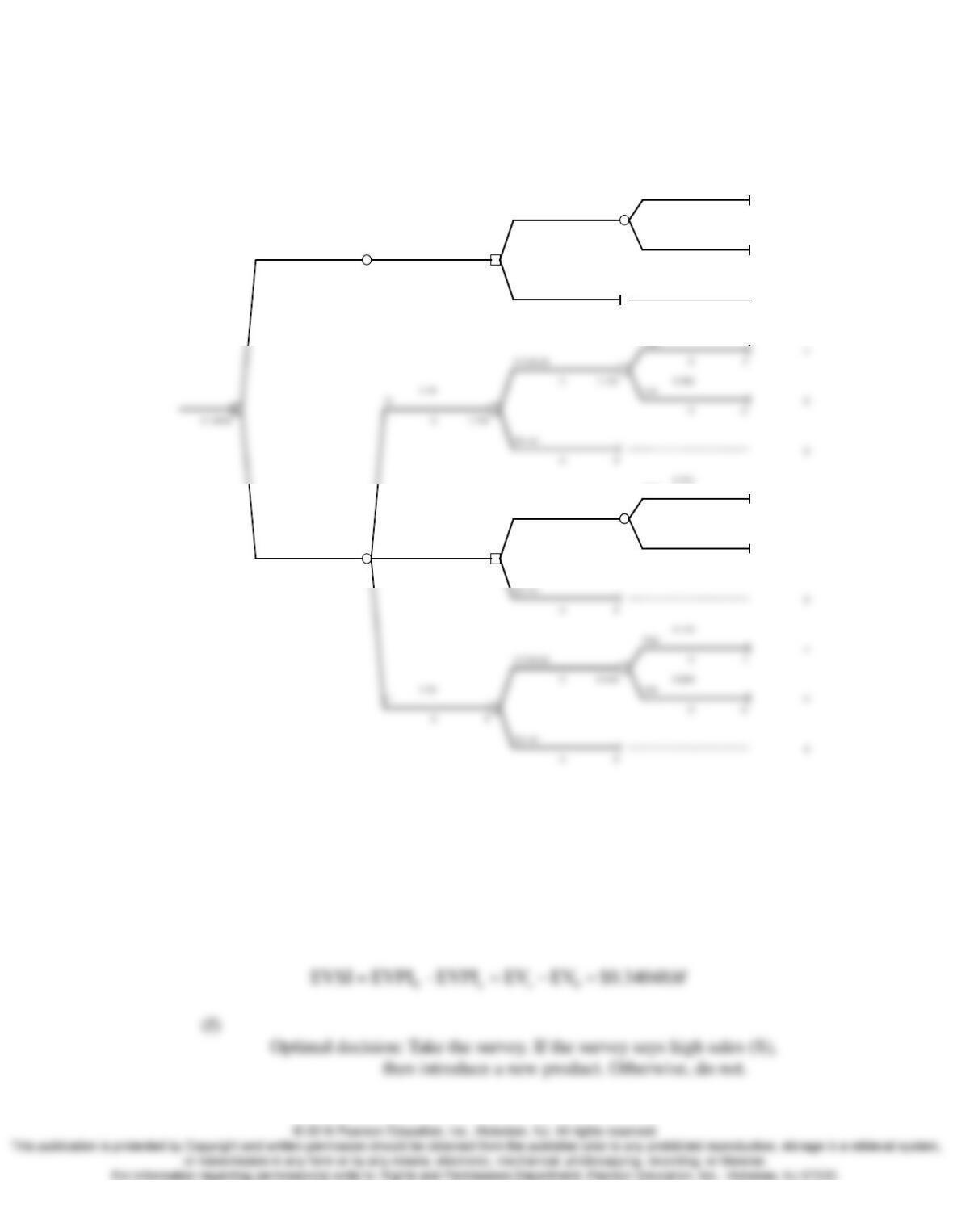
(c) Decision tree
(d)
EVPI EPPI EV $1.2 $0.34048 $0.85952
ee
MM M= −= − =
(e)
0. 3
High
4
int roduce 0 4
0– 0 .2 0 .7
1Low
No surv ey Event 3 – 2
2 0 – 2
0 0 0 0
Do not
0
0 0
0.6 32
High
High
4
int roduce 0 4
0–0.4 7 0.745
0.4 7 Low
Do sur vey I– 2
2 0 – 2
– 0 .2 0.34048 0 0
12.26
(a) Let’s define the symbols:
P: Party is taking place
(b)
• Optimal decision without sample information:
• Joint & Marginal probabilities:
Tipster says
Marginal
Probability
TP
TNP
• Conditional probabilities:
Tipster says
TP
TNP
• Optimal decision after receiving the tips:
The tipster’s information has no value, even though it costs nothing.
Do not reply on the tips.
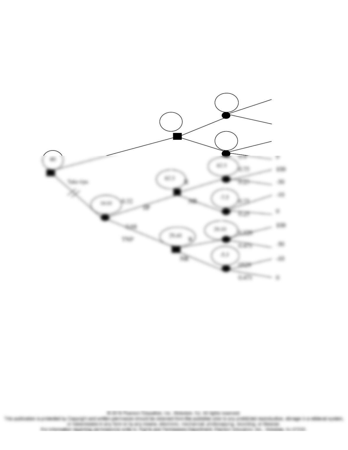
* Decision Tree
R
NR
40
100
-50
-10
0.6
0.4
0.6
40
-6
Do not take tips
R
R
NR
62.5
0
100
-50
-10
0
100
-50
-10
0
0.4
0.75
0.25
0.75
0.25
0.529
0.471
0529
0.471
62.5
29.41
0.32
0.68
40
12.27
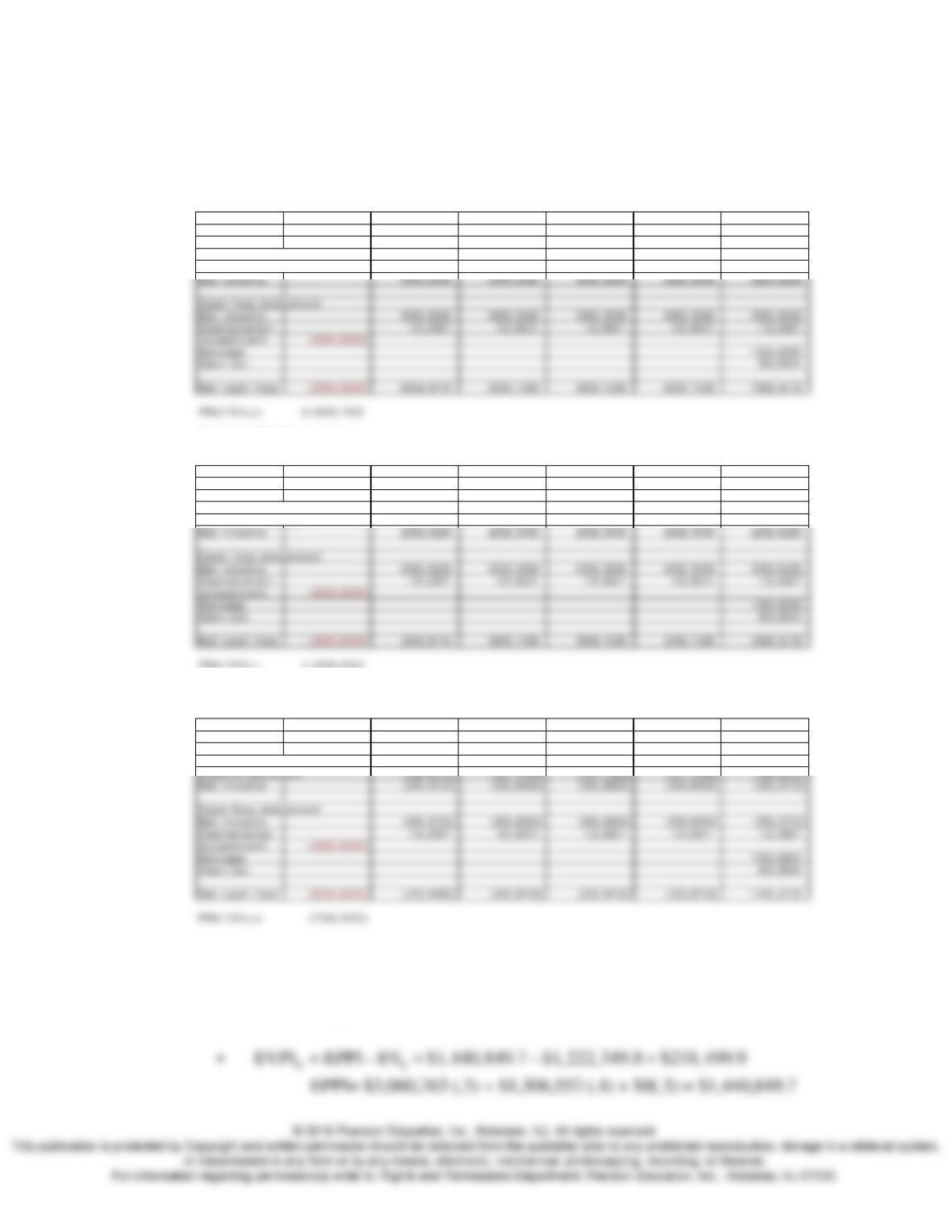
(a)
0
EV (0.3)($3,060,763) (0.4)($1,306,552) (0.3)( $728,333)
$1, 222,349.8
= + +−
=
Open the store
De m an d H igh ca se
I ncom e st at em e nt
0 1 2 3 ... 1 4 15
Revenue 1,000,000 1,000,000 1,000,000 1,000,000 1,000,000
Depreciation 12,287 1 2,821 12,821 12,821 12,287
taxable incom e 987,7 14 987,180 987,180 987,180 987,714
incom e t ax (40% ) 395,0 85 394,872 394,872 394,872 395,085
De m an d M ediu m ca se
I ncom e st at em e nt
0 1 2 3 ... 1 4 15
Revenue 500,000 50 0,000 500,000 500,000 500,000
Depreciation 12,287 1 2,821 12,821 12,821 12,287
taxable incom e 487,7 14 487,180 487,180 487,180 487,714
incom e t ax (40% ) 195,0 85 194,872 194,872 194,872 195,085
PW( 1 5 % ) = 1,306,552
De m a n d Low case
I ncom e st at em e nt
0 1 2 3 ... 1 4 15
Revenue (80,000) (80 ,000) (80,000) (80,000) (80,000)
Depreciation 12,287 1 2,821 12,821 12,821 12,287
taxable incom e (92,287) (92,821) (92,82 1) (92,821) (92,287)