Economics Chapter 12 Keynesian Business Cycle Analysis Nonmarket clearing

Keynesian Business Cycle Analysis: Non–Market–Clearing Macroeconomics 235

of changing prices may exceed the additional profit earned from doing so. A

5. In the Keynesian model, money is not neutral in the short run, but it is neutral in the

long run. In the short run, an increase in the money supply increases output and

the real interest rate, while the price level and real (efficiency) wage are

unchanged. In the long run, however, only the price level is changed, with no

6. In the Keynesian model in the short run, output and the real interest rate increase

due to an increase in government purchases. In the long run, the real interest rate

is higher, but output returns to its full-employment level. Since the real interest rate

is higher in the long run, investment is lower and consumption is lower.

7. In response to a recession, policymakers can (1) make no change in

macroeconomic policy (2) increase the money supply, or (3) increase government

purchases.

If they make no change in macroeconomic policy, then during the recession output

is below its full-employment level. Over time, the price level will decline to restore

8. Employment is procyclical because a contractionary aggregate demand shock

reduces both output and employment. Money is procyclical because price

stickiness means that an increase in the money supply increases output as the

236 Chapter 12

9. The Keynesian theory assumes that demand shocks cause most cyclical

fluctuations. This means that during expansions when employment rises, average

10. In Keynesian analysis, a supply shock may reduce output in two ways: (1) a

reduction in output, because the supply shock reduces the marginal product of

labour, shifting the FE line to the left; and (2) a further reduction in output if the

Numerical Problems

1. a. Setting w = MPN, w = 10 / . This is the labour demand curve.

b. At W = 20, w = W/P = 20/P. Since labour demand is given by w = 10 / ,

then 20/P = 10 or 2 =

P.

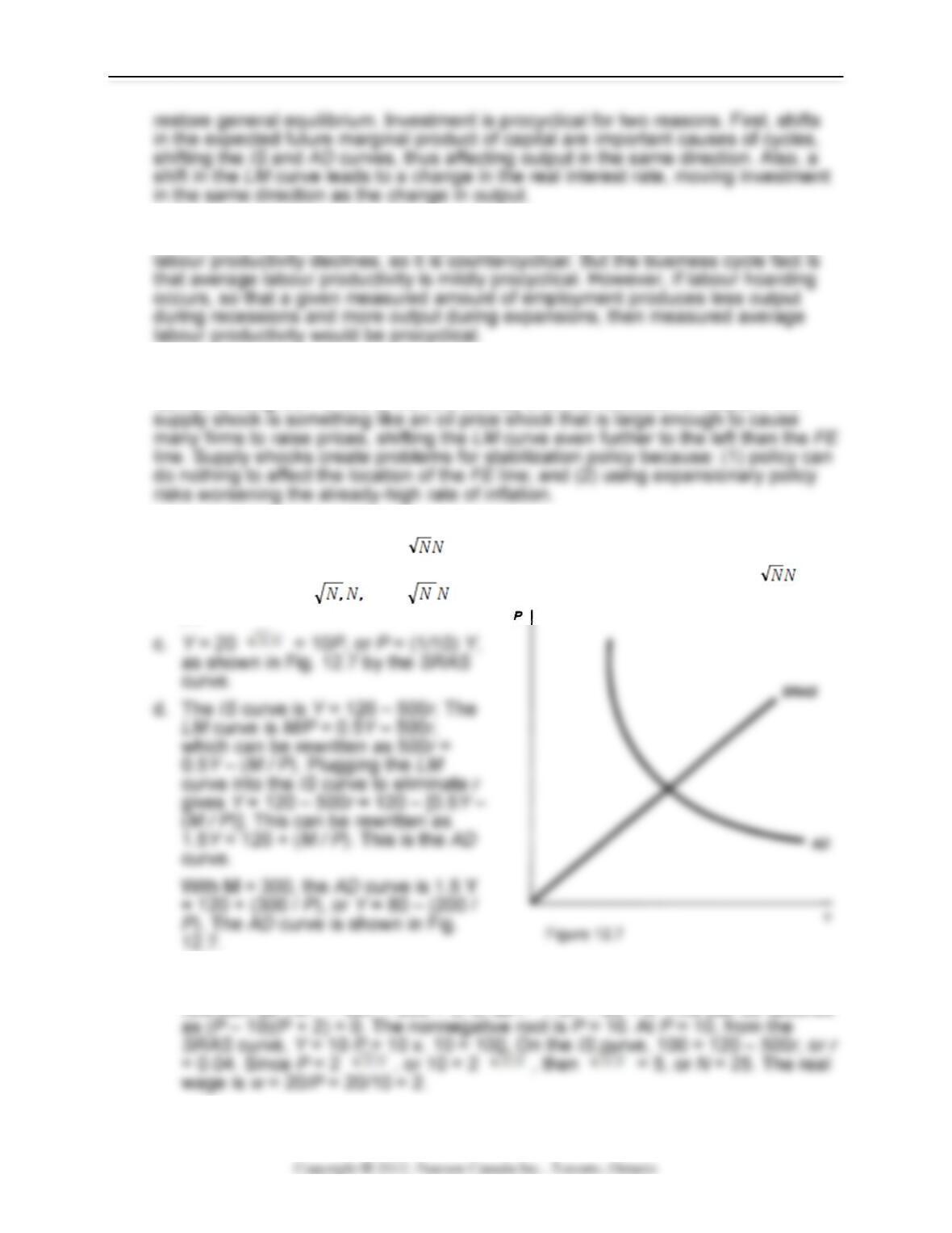
e. To find the intersection of the SRAS curve (Y = 10/P) and the AD curve [Y = 80

+ (200 / P)], find the price level such that 10P = 80 + (200 / P). This can be

rewritten as 10P2 = 80P – 200 = 0, or as P2 – 8P – 20 = 0. This can be factored

Keynesian Business Cycle Analysis: Non–Market–Clearing Macroeconomics 237

f. When the money supply falls to 135, the AD curve becomes 1.5Y = 120 = (135

2. a. The IS curve is found from the equation Y = Cd + Id + G = 130 – 0.5(Y – 100) –

500r – 100 – 500r + 100, or 0.5Y = 280 – 1000r, or Y = 560 – 2000r.

The LM curve comes from the equation M/P = L, which in this case is 1320 / P

= 0.5Y – 1000r, or Y – (2640/P) + 2000r.

c. If desired investment increases to

200 – 500r, the IS curve shifts from

IS1 to IS2 in Fig. 12.8. This can be

seen in the equation Y = Cd – Id – G

= 130 + 0.5(Y – 100) – 500r + 200 –

500r + 100, or 0.5Y = 380 – 1000r,

3. The IS curve is Y = Cd + Id + G = 325 + 0.5(Y – 150) – 500r + 200 – 500r + G =

450 + 0.5Y – 1000r + G. This can be rewritten as 0.5Y = 450 – 1000r + G, or Y =

900 – 2000r + 2G. The LM curve is M/P = L = 0.5Y – 1000r.

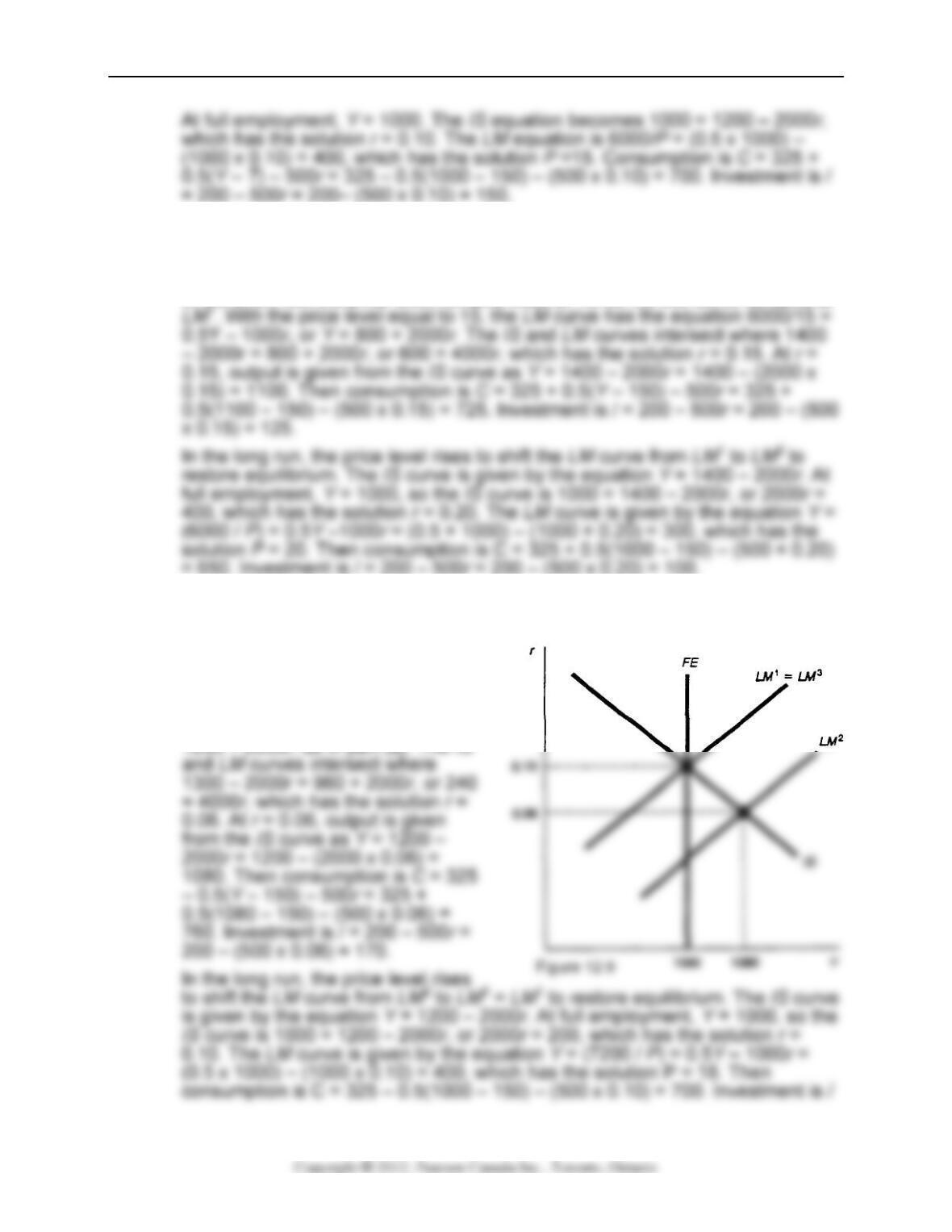
a. When G = 150, the IS curve is Y = 900 – 2000r + (2 x 150) = 1200 – 2000r.

With M = 6000, the LM curve is 6000/P = 0.5Y – 1000r.

238 Chapter 12

b. When G increases to 250, the IS curve shifts from IS1 to IS2 in Fig. 13.11. The

new IS equation is Y = 900 – 2000r + 2G = 900 – 2000r + (2 x 250) = 1400 –

2000r.

In the short run, the price level remains fixed at 15, so the LM curve remains at

c. When the money supply increases to 7200, the LM curve shifts from LM1 to

LM2 in Fig. 12.9. The LM equation is 7200 / P + 0.5Y – 1000r.

In the short run, the price level

remains fixed at 15, so the LM

curve has the equation 7200 / 15 =

0.5Y – 1000r, or Y = 960 + 2000r.

The IS curve has the equation Y =

Keynesian Business Cycle Analysis: Non–Market–Clearing Macroeconomics 239

4. The IS curve is Y = Cd + Id + G = [600 + 0.8(Y − 1000) − 500r] +[400 − 500r]+

1000, so 0.2Y = 1200 − 1000r.

Since πe= 0, the nominal interest rate (i) equals the real interest rate (r).

a. Can the economy reach full employment? Since full-employment output is Y =

b. To restore full employment while the nominal interest rate is zero clearly

requires a shift in the IS curve. If we return to the original derivation and put G

in the equation instead of using the original value of G = 1000, we get:

5. a. The IS curve is given by Y = Cd + Id + G + NX = 120 + 0.5(Y – 100) + 120 –

200r + 100 + 60 + 0.5YFOR = 100r = 400 + 0.5Y – 500r. This can be rewritten as

b. With P = 18, the AD curve is Y = 160 + (10 800/18) = 760. From the IS curve,

760 = 800 –1000r, which has the solution r = 0.04. Consumption is C = 120 +

0.5(760 – 100) – (200 x 0.04) = 442. Investment is / = 120 – (200 x 0.04) = 112.

c. In the long run, Y = 700. From the IS equation, 700 = 800 – 1000r, which has

240 Chapter 12

6. The following table shows the real wage (w), the effort level (E), and the effort per

unit of real wages (E / w).

w E E / w

8 7 0.875

7. a. Using the definition, in Appendix 9.A, αIS = 0.6, βIS = 0.0005, αLM = 0, βLM =

0.0005, and ℓr = 1000.

Keynesian Business Cycle Analysis: Non–Market–Clearing Macroeconomics 241

Analytical Problems

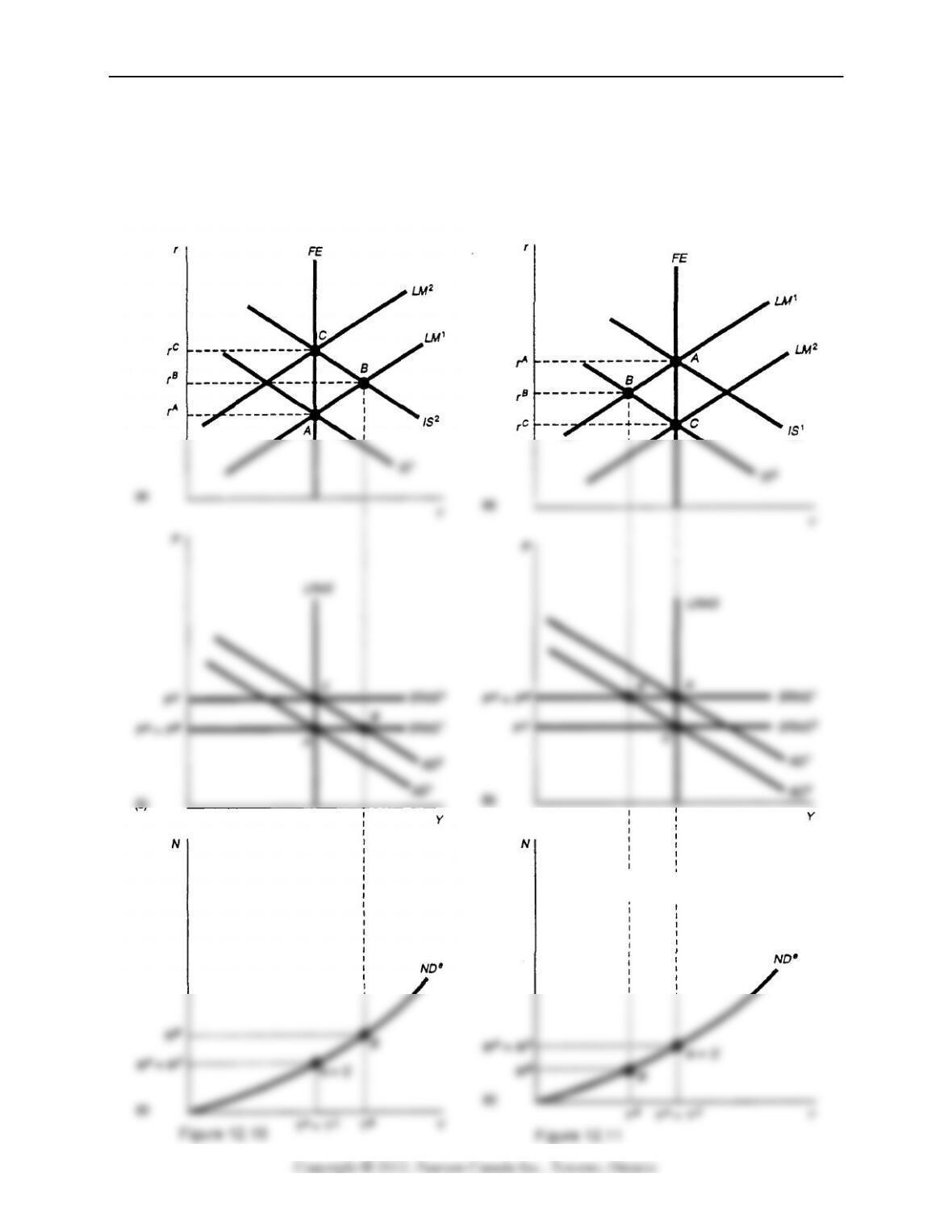
1. In Figs. 12.10 and 12.11, point A is the starting point, point B shows the short-run

equilibrium after the change, and point C shows the long-run equilibrium after the

change.

Figure 12.10

Figure 12.9

242 Chapter 12

a. In Fig. 12.10, the increase in tax incentives increases investment, shifting the IS

curve to the right from IS1 to IS2 in Fig. 12.10(a), and shifting the AD curve from

AD1 to AD2 in Fig. 12.10(b). The short-run equilibrium is at point B. Output

increases, the real interest rate

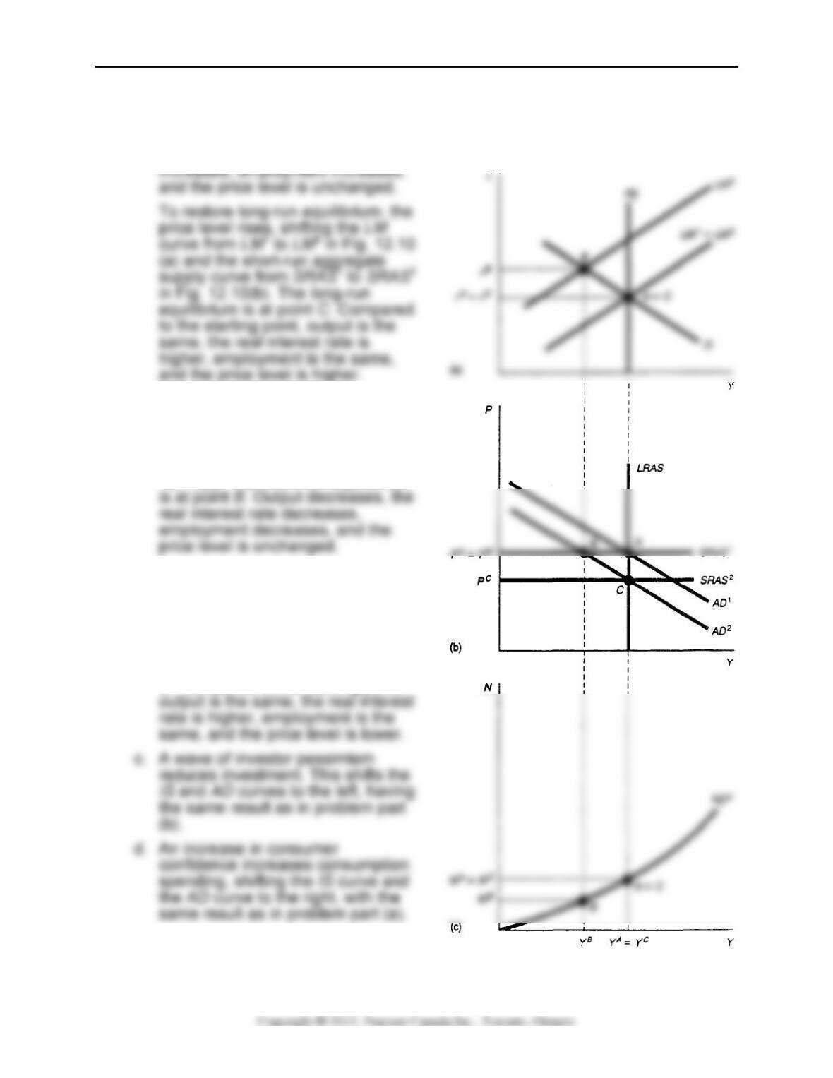
b. In Fig. 12.11, the increase in tax

incentives increases saving—

shifting the IS curve from IS1 to IS2

in Fig. 12.11(a), and shifting the AD

curve from AD1 to AD2 in Fig.

12.11(b). The short-run equilibrium

To restore long-run equilibrium, the

price level rises, shifting the LM

curve from LM1 to LM2 in Fig.

12.11(a) and the short-run

aggregate supply curve from

SRAS1 to SRAS2 in Fig. 12.11(b).

The long-run equilibrium is at point

C. Compared to the starting point,

2. In Figs. 12.12–12.15, point A is the

starting point, point B shows the short-

Figure 12.12

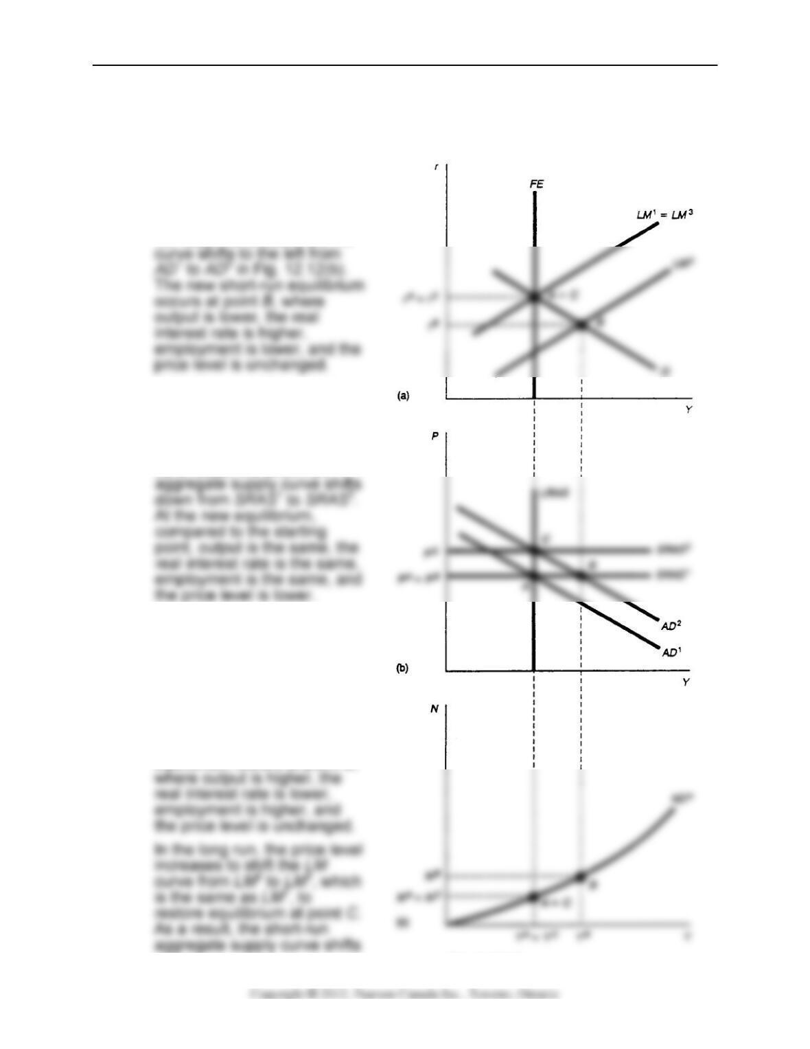
Figure 12.15

Keynesian Business Cycle Analysis: Non–Market–Clearing Macroeconomics 243

run equilibrium after the change, and point C shows the long-run equilibrium after

the change.

a. In Fig. 12.12, when bank

pays a higher interest rate on

chequing accounts, the

demand for money rises,

shifting the LM curve to the

left from LM1 to LM2 in Fig.

12.12(a). As a result, the AD

In the long run, the price level

decreases to shift the LM

curve from LM2 to LM1, which

is the same as LNP, to

restore equilibrium at point C.

As a result, the short-run

b. In Fig. 12.13, the introduction

of credit cards reduces the

demand for money—shifting

the LM curve to the right from

LM1 to LM2 in Fig. 12.13(a).

As a result, the AD curve

shifts from AD1 to AD2 in Fig.

12.13(b). The new short-run

equilibrium occurs at point B,

Figure 12.13

244 Chapter 12

up from SRAS1 to SRAS2. At the new equilibrium, compared to the starting

point, output is the same, the real interest rate is the same, employment is the

same, and the price level is

higher.

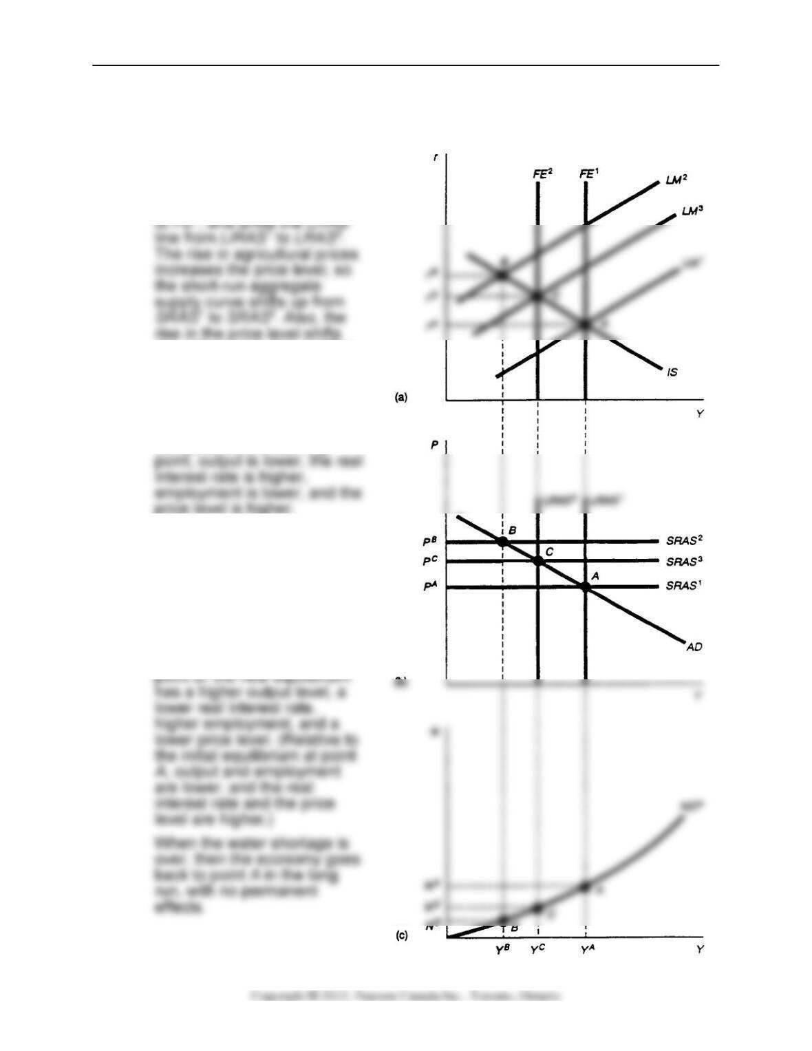
c. In Fig. 12.14, the reduction in

agricultural output shifts the

FE curve to the left from FE1

the LM curve up from LM1 to

LM2. The short-run

equilibrium is at point B,

assuming that the LM curve

shifts to the left more than

the FE line. At point B,

compared to the starting

price level is higher.

If the water shortage persists,

a new long-run equilibrium

occurs at points C. To get to

this equilibrium, the price

level must decline, shifting

the LM curve from LM2 to

LM3, and the short-run

aggregate supply curve from

SRAS2 to SRAS3. Relative to

Figure 12.14

Keynesian Business Cycle Analysis: Non–Market–Clearing Macroeconomics 245

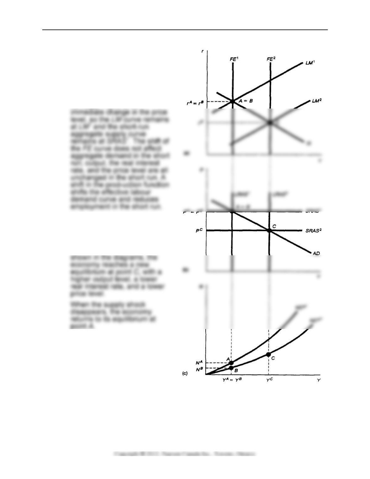
d. In Fig. 12.15, the beneficial

supply shock makes more

production possible at full

employment, so the FE line

shifts to the right in Fig.

12.15(a) from FE1 to FE2, and

the LRAS line shifts from

LRAS1 to LRAS2 in Fig.

12.15(b). There is no

If the supply shock persists,

prices will decline, so the LM

curve will shift from LM1 to LM2

and the SRAS curve will shift

from SRAS1 to SRAS2. As

3. A lag in the impact of policy of six

months, which is about the time it

takes firms to adjust prices, could

cause policy to be destabilizing.

That is, monetary policy may be

pushing the economy away from

equilibrium.

Figure 12.15

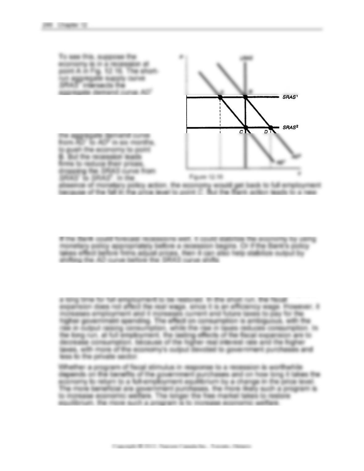
at point A, to the left of the

long-run aggregate supply

curve LRAS. Suppose the

Bank engages in expansionary

monetary policy to try to shift

equilibrium at point D. So the Bank causes the economy to overshoot the

equilibrium point. The result may be to exaggerate the business cycle, pushing

output too high in expansions. Then if the Bank responds to an expansion by using

contractionary monetary policy, it may overshoot on the other side, causing a new

recession.

4. An increase in government purchases shifts the IS and AD curves to the right to

return the economy to full employment, instead of waiting for the price level to fall

to get there. The advantage of doing so, according to Keynesians, is that full

employment is restored quickly, whereas if the price level must adjust, it may take

5. a. In response to expansionary monetary policy, aggregate demand increases,

increasing output and labour demand. This causes the labour demand curve to

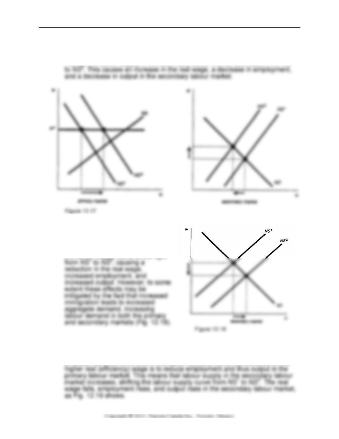
Keynesian Business Cycle Analysis: Non–Market–Clearing Macroeconomics 247

shift from ND1 to ND2 in the primary labour market, shown in Fig. 12.17. The

result is an increase in employment and output with no change in the real wage

in the primary labour market. Since more workers are now in the primary labour

market, the labour supply in the secondary labour market decreases from NS1

b. Increased immigration has no effect

in the primary labour market, since

labour supply changes in general

have no effect. In the secondary

labour market, the immigration shifts

the labour supply curve to the right

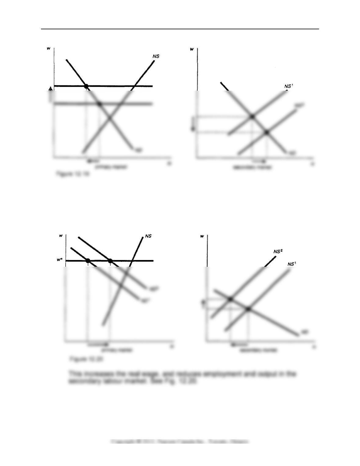
c. If there is a shift in the effort curve, the efficiency wage rises in the primary

labour market. Since effort exerted at the higher wage is the same as before

the change, the shift in the effort curve has no impact on the marginal product

of labour, so there is no shift in the labour demand curve. So the effect of the

248 Chapter 12

d. The productivity improvement shifts the labour demand curve to the right, so at

the fixed real (efficiency) wage, firms demand more labour. Employment

increases, so output increases in the primary labour market. The increase in

employment in the primary labour market reduces the labour supply in the

secondary labour market, shifting the labour supply curve from NS1 to NS2.

Keynesian Business Cycle Analysis: Non–Market–Clearing Macroeconomics 249

e. The productivity improvement in the secondary labour market has no effect on

the primary labour market. In the secondary labour market, increased