Economics Chapter 12 Interactive Activity Aggregate Demand And Aggregate Supply Fall The Value The

Unlock access to all the studying documents.

View Full Document

S-161

interactive activity

Chapter 12

Aggregate Demand and

Aggregate Supply

1. A fall in the value of the dollar against other currencies makes U.S. final goods

and services cheaper to foreigners even though the U.S. aggregate price level

stays the same. As a result, foreigners demand more American aggregate output.

Your study partner says that this represents a movement down the aggregate

demand curve because foreigners are demanding more in response to a lower

price. You, however, insist that this represents a rightward shift of the aggregate

demand curve. Who is right? Explain.

1. You are right. When a fall in the value of the dollar against other currencies

2. Your study partner is confused by the upward-sloping short-run aggregate

supply curve and the vertical long–run aggregate supply curve. How would you

explain this?

3. Suppose that in Wageland all workers sign annual wage contracts each year on

January1. No matter what happens to prices of final goods and services dur-

ing the year, all workers earn the wage specified in their annual contract. This

year, prices of final goods and services fall unexpectedly after the contracts are

signed. Answer the following questions using a diagram and assume that the

economy starts at potential output.

a. In the short run, how will the quantity of aggregate output supplied respond

to the fall in prices?

b. What will happen when firms and workers renegotiate their wages?

Solution

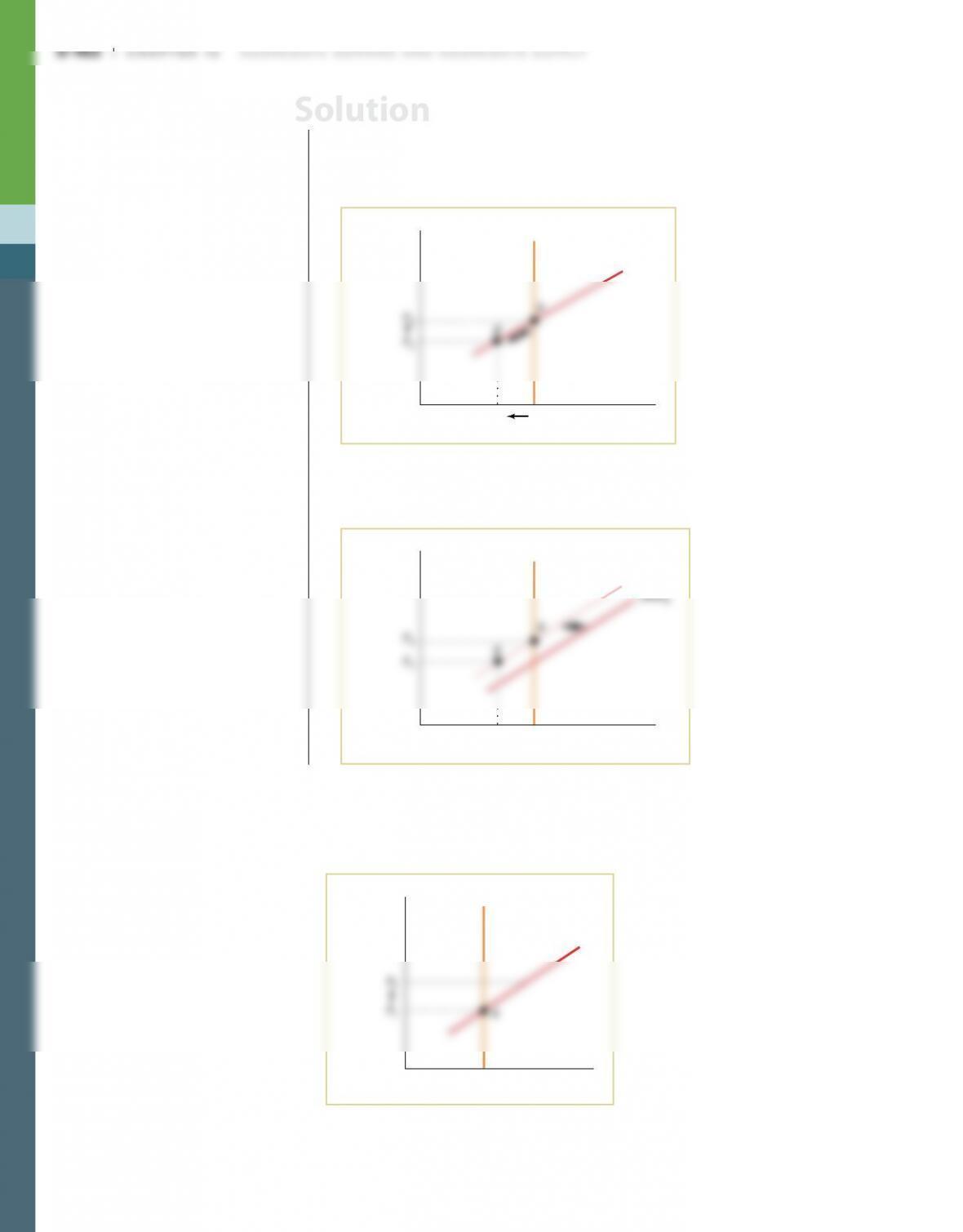
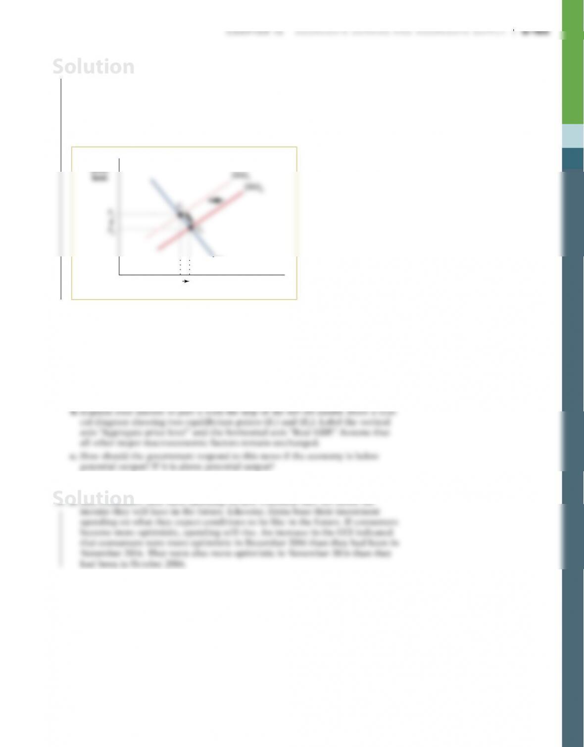
3. a. In the short run, the prices of final goods and services in Wageland fall

unexpectedly but nominal wages don’t change; they are fixed in the short

run by the annual contract. So firms earn a lower profit per unit and reduce

output. In the accompanying diagram, Wageland moves along SRAS1 from

point A on January 1 to point B after the fall in prices.

Aggregate

price

level

Real GDPYP

LRAS

SRAS

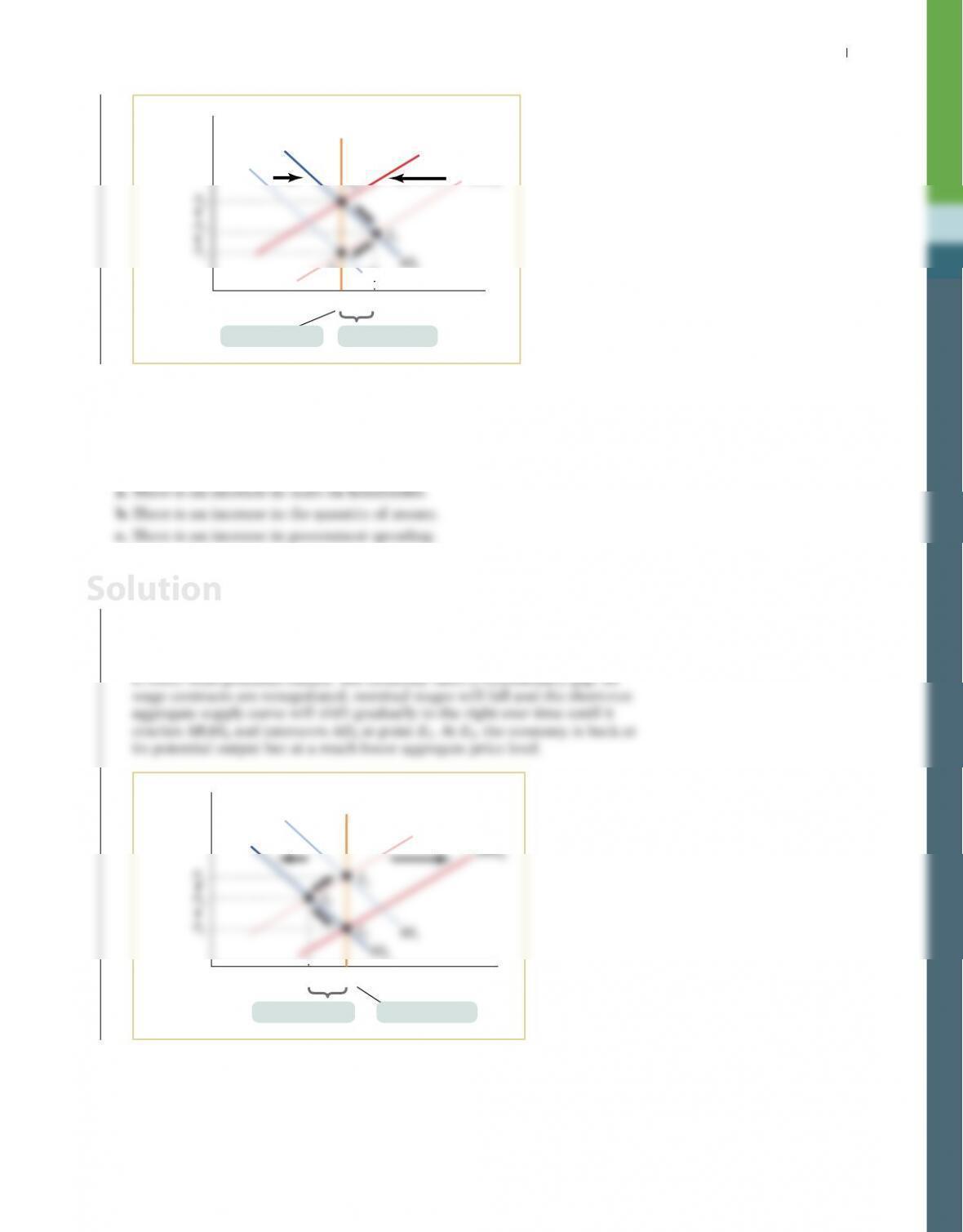
b. When firms and workers renegotiate their wages, nominal wages will

decrease, shifting the short–run aggregate supply curve in the accompanying

diagram rightward from SRAS1 to a curve such as SRAS2.

Aggregate

price

level

Real GDPY

LRAS

SRAS1

4. The economy is at point A in the accompanying diagram. Suppose that the

aggregate price level rises from P1 to P2. How will aggregate supply adjust in the

short run and in the long run to the increase in the aggregate price level? Illus–

trate with a diagram.

Real GDP

ggregate

price

level

LRAS

SRAS1

Solution

4. In the short run, as the aggregate price level rises from P1 to P2, nominal wages

will not change. So profit per unit will rise, leading to an increase in production

from Y1 to Y2. The economy will move from point A to point B in the accompa-

nying diagram. In the long run, however, nominal wages will be renegotiated

upward in reaction to low unemployment at Y2. As nominal wages increase,

the short–run aggregate supply curve will shift leftward from SRAS1 to a posi-

tion such as SRAS2. The exact position of SRAS2 depends on factors such as the

aggregate demand curve.

Aggregate

price

Real GDPY2

LRAS

SRAS2

5. Suppose that all households hold all their wealth in assets that automatically

rise in value when the aggregate price level rises (an example of this is what is

called an “inflation–indexed bond”—a bond whose interest rate, among other

things, changes one–for–one with the inflation rate). What happens to the wealth

effect of a change in the aggregate price level as a result of this allocation of

assets? What happens to the slope of the aggregate demand curve? Will it still

slope downward? Explain.

5. If all households hold all their wealth in assets that automatically rise in value

when the aggregate price level rises, this will eliminate the wealth effect of a

change in the aggregate price level. The purchasing power of consumers’ wealth

will not vary with a change in the aggregate price level, so there will be no

change in consumer spending due to the change in the aggregate price level. The

aggregate demand curve will still slope downward because of the interest rate

6. Suppose that the economy is currently at potential output. Also suppose that you

are an economic policy maker and that a college economics student asks you to

rank, if possible, your most preferred to least preferred type of shock: positive

demand shock, negative demand shock, positive supply shock, negative supply

shock. How would you rank them and why?

Solution

S-164 Chapter 12 AggregAte DemAnD AnD AggregAte Supply

6. The most preferred shock would be a positive supply shock. The economy would

have higher aggregate output without the danger of inflation. The government

would not need to respond with a change in policy. The least preferred shock

would be a negative supply shock. The economy would experience stagflation.

There would be lower aggregate output and higher inflation. There is no good

policy remedy for a negative supply shock: policies to counteract the slump in

7. Explain whether the following government policies affect the aggregate demand

curve or the short–run aggregate supply curve and how.

7. a. If the government reduces the minimum nominal wage, it is similar to a fall

in nominal wages. Aggregate supply will increase, and the short–run aggregate

supply curve will shift to the right.

b. If the government increases TANF, consumer spending will increase because

disposable income increases (disposable income equals income plus govern-

ment transfers, such as TANF payments, less taxes). Aggregate demand will

increase, and the aggregate demand curve will shift to the right.

8. In Wageland, all workers sign annual wage contracts each year on January 1. In

late January, a new computer operating system is introduced that increases labor

Solution

8. As labor productivity increases, producers will experience a reduction in produc-

tion costs and profit per unit of output will increase. Producers will respond by

increasing the quantity of aggregate output supplied at any given aggregate price

level. The short-run aggregate supply curve will shift to the right. Beginning at

short–run equilibrium, E1 in the accompanying diagram, the short-run aggregate

supply curve will shift from SRAS1 to SRAS2. The aggregate price level will fall,

and real GDP will increase in the short run.

Real GDPY2

Aggregate

price

9. The Conference Board publishes the Consumer Confidence Index (CCI) every

month based on a survey of 5,000 representative U.S. households. It is used

by many economists to track the state of the economy. A press release by the

Board on December 27, 2016, stated: “The Conference Board Consumer Confi-

dence Index®, which had increased considerably in November, posted another

gain in December. The Index now stands at 113.7 (1985 = 100), up from 109.4 in

November.”

a. As an economist, is this news encouraging for economic growth?

9. a. Yes, consumers base their spending on how confident they are about the

Solution

S-166 Chapter 12 AggregAte DemAnD AnD AggregAte Supply

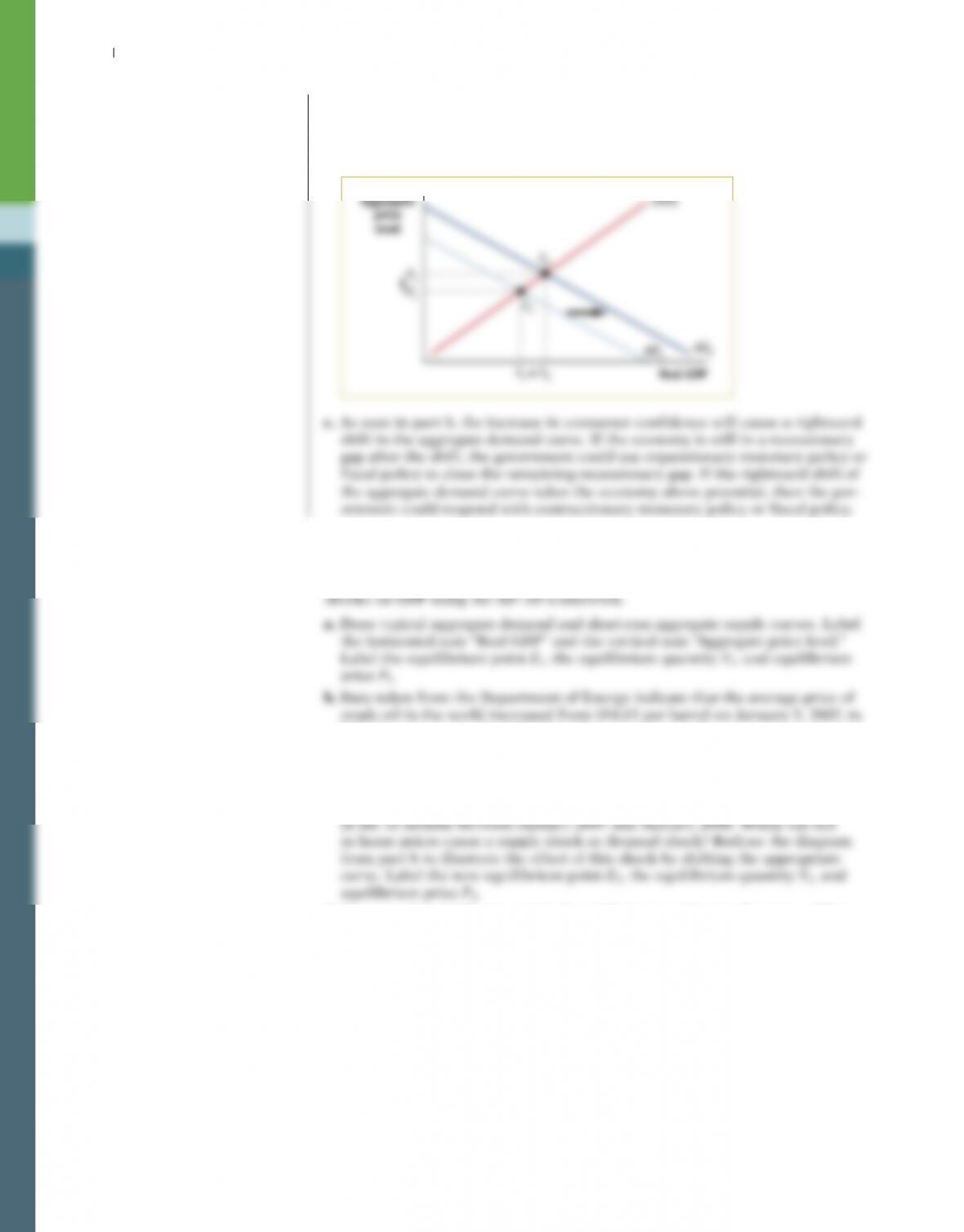
b. An increase in consumer confidence leads to a rightward shift of the aggre–

gate demand curve. As shown, in the accompanying diagram, other things

equal, this will increase real GDP from Y1 to Y2 and will increase the aggregate

price level from P1 to P2.

AD1 AD

SRAS

Y1Real GDP

Aggregate

price

level

c. As seen in part b, the increase in consumer confidence will cause a rightward

shift in the aggregate demand curve. If the economy is still in a recessionary

gap after the shift, the government could use expansionary monetary policy or

fiscal policy to close the remaining recessionary gap. If the rightward shift of

the aggregate demand curve takes the economy above potential, then the gov-

ernment could respond with contractionary monetary policy or fiscal policy.

10. There were two major shocks to the U.S. economy in 2007, leading to the severe

recession of 2007–2009. One shock was related to oil prices; the other was the

slump in the housing market. This question analyzes the effect of these two

$92.93 on December 28, 2007. Would an increase in oil prices cause a demand

shock or a supply shock? Redraw the diagram from part a to illustrate the

effect of this shock by shifting the appropriate curve.

c. The Housing Price Index, published by the Office of Federal Housing Enter-

prise Oversight, calculates that U.S. home prices fell by an average of 3.0%

d. Compare the equilibrium points E1 and E3 in your diagram for part c. What

was the effect of the two shocks on real GDP and the aggregate price level

(increase, decrease, or indeterminate)?

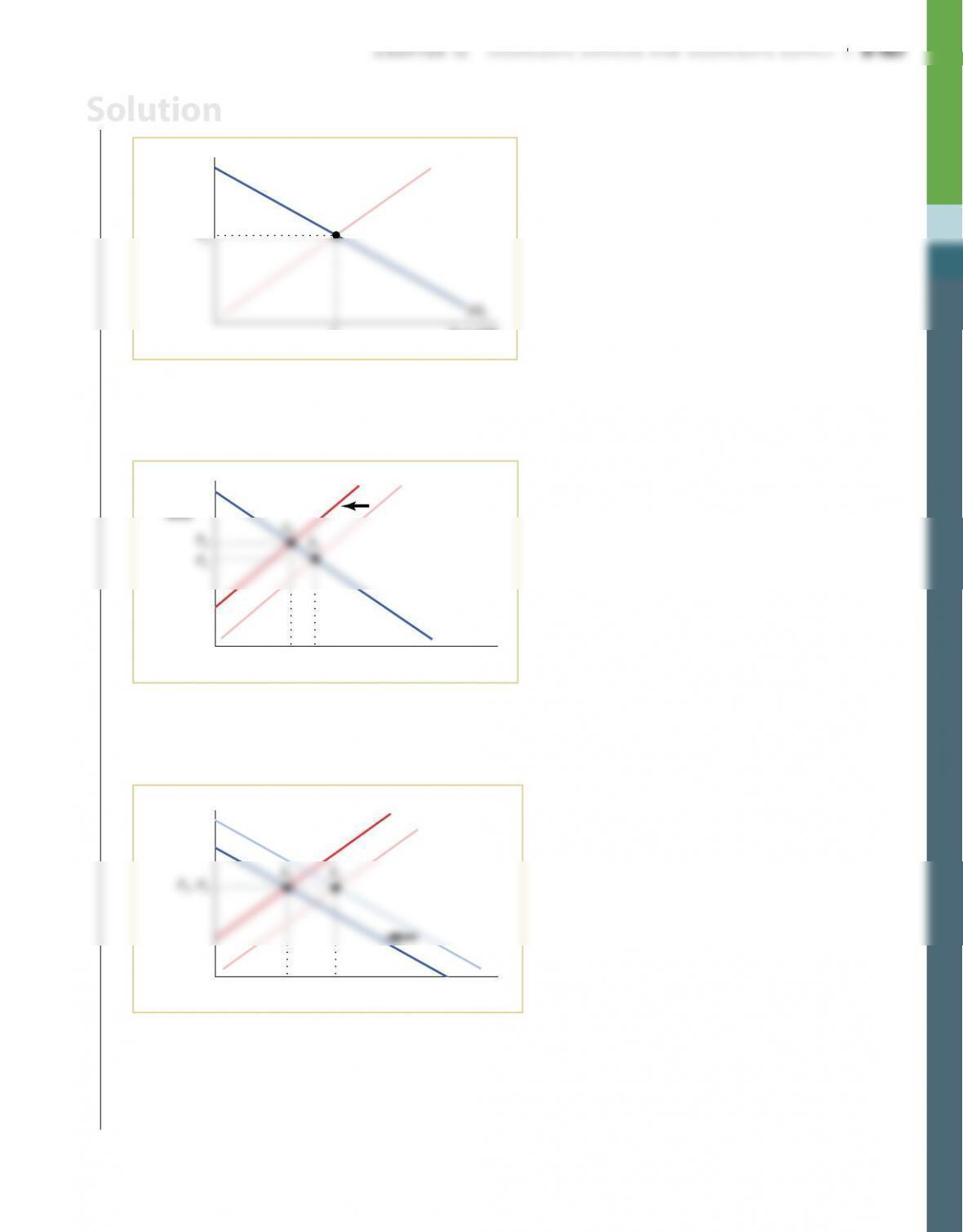
10. a. The graph will look like this:

SRAS

Real GDP

Aggregate

price

level

b. The rise in the price of oil usually causes a supply shock. The short-run aggre–

gate supply (SRAS) curve shifts to the left, from SRAS1 to SRAS2. The economy

settles at a new short-run macroeconomic equilibrium at E2, with a higher

aggregate price level, P2, and lower real GDP, Y2.

SRAS

AD1

Real GDP

Aggregate

price

level

P2E1

c. The fall in home prices would cause a demand shock because of the wealth

effect. The aggregate demand (AD) curve shifts leftward, from AD1 to AD2. The

new aggregate price level, P3, could either be equal to, above, or below P1. The

new level of real GDP, Y3, is below the original level, Y1.

SRAS

SRAS1

AD2 AD

Real GDP

ggregate

price

level

d. The effect on the aggregate price level is indeterminate. As drawn in the

diagram for part c, P1 and P3 coincide because the negative supply and

demand shocks have exactly offsetting price effects. However, prices could

either rise or fall when both a negative demand shock and a negative supply

shock occur. The fall in real GDP is unambiguous because the two shocks

reinforce their negative effects on GDP.

Solution

11. Using aggregate demand, short–run aggregate supply, and long–run aggregate

supply curves, explain the process by which each of the following economic

events will move the economy from one long–run macroeconomic equilibrium

toanother. Illustrate with diagrams. In each case, what are the short–run and

long–run effects on the aggregate price level and aggregate output?

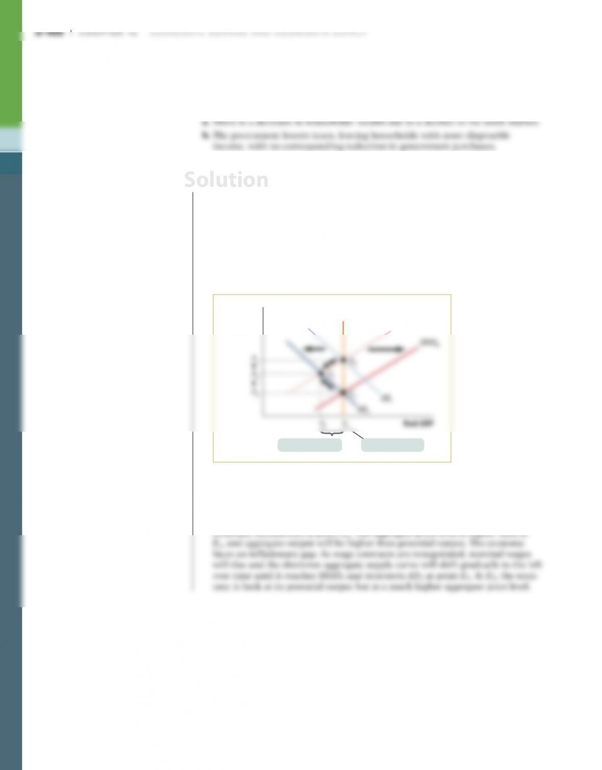
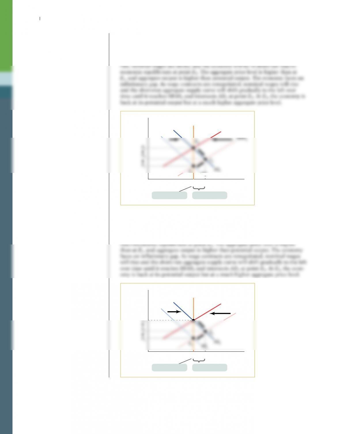
11. a. A decrease in households’ wealth will reduce consumer spending. Beginning

at long–run macroeconomic equilibrium, E1 in the accompanying diagram, the

aggregate demand curve will shift from AD1 to AD2. In the short run, nomi–

nal wages are sticky, and the economy will be in short–run macroeconomic

equilibrium at point E2. The aggregate price level will be lower than at E1, and

aggregate output will be lower than potential output. The economy faces a

recessionary gap. As wage contracts are renegotiated, nominal wages will fall

and the short–run aggregate supply curve will shift gradually to the right over

time until it reaches SRAS2 and intersects AD2 at point E3. At E3, the economy

is back at its potential output but at a much lower aggregate price level.

Aggregate

price

level

LRAS

SRAS1

SRAS

Solution

Chapter 12 AggregAte DemAnD AnD AggregAte Supply S-169

Aggregate

price

level

Real GDPY2

LRAS

SRAS

SRAS2

Inflationary gapPotential output

AD1

12. Using aggregate demand, short–run aggregate supply, and long–run aggregate

supply curves, explain the process by which each of the following government

policies will move the economy from one long–run macroeconomic equilibrium

to another. Illustrate with diagrams. In each case, what are the short–run and

long–run effects on the aggregate price level and aggregate output?

12. a. An increase in taxes will decrease consumer spending by households.

Beginning at E1 in the accompanying diagram, the aggregate demand curve

will shift leftward from AD1 to AD2. In the short run, nominal wages are

sticky, and the economy will be in short–run macroeconomic equilibrium at

point E2. The aggregate price level is lower than at E1, and aggregate output

Aggregate

price

level

LRAS

SRAS1

SRAS

Solution

S-170 Chapter 12 AggregAte DemAnD AnD AggregAte Supply

b. An increase in the quantity of money will encourage people to lend, lowering

interest rates and increasing investment and consumer spending; at any given

aggregate price level, the quantity of aggregate output demanded will be higher.

Beginning at long–run macroeconomic equilibrium, E1 in the accompanying

diagram, the aggregate demand curve will shift from AD1 to AD2. In the short

Aggregate

price

level

Real GDPY2

LRAS

SRAS2

Inflationary gapPotential output

AD1

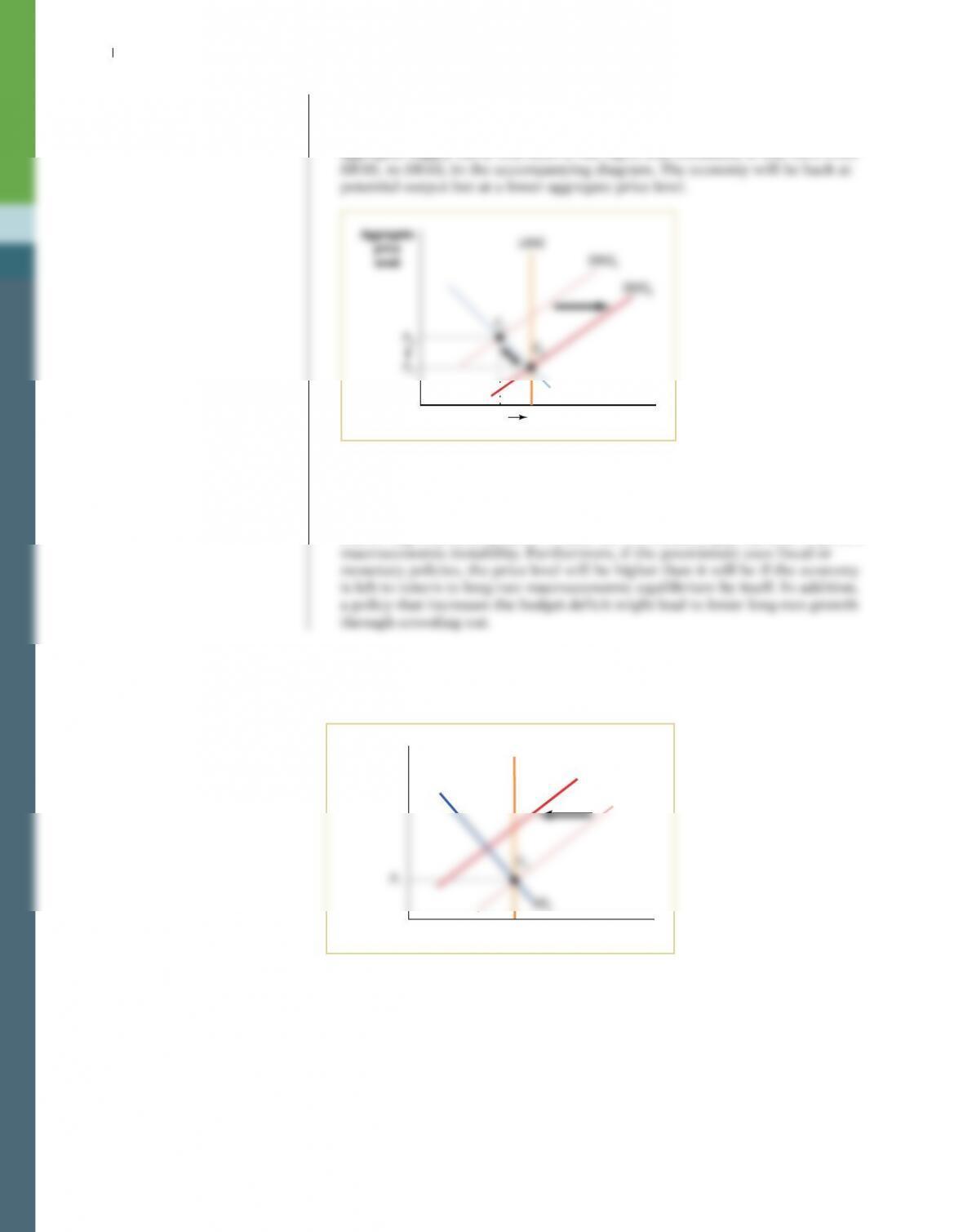
c. An increase in government spending will increase aggregate demand; at any

given aggregate price level, the quantity of aggregate output demanded will be

higher. Beginning at long–run macroeconomic equilibrium, E1 in the accom–

panying diagram, the aggregate demand curve will shift from AD1 to AD2. In

the short run, nominal wages are sticky, and the economy will be in short-run

Aggregate

price

level

Real GDPY2

LRAS

SRAS

SRAS2

Inflationary gapPotential output

13. The economy is in short–run macroeconomic equilibrium at point E1 in the

accompanying diagram. Based on the diagram, answer the following questions.

Real GDP

ggregate

price

level

LRAS

SRAS

AD1

a. Is the economy facing an inflationary or a recessionary gap?

b. What policies can the government implement that might bring the economy

back to long–run macroeconomic equilibrium? Illustrate with a diagram.

c. If the government did not intervene to close this gap, would the economy

return to long–run macroeconomic equilibrium? Explain and illustrate with a

13. a. The economy is facing a recessionary gap because Y1 is less than the potential

output of the economy, YP.

b. The government could use either fiscal policy (increases in government spend-

ing or reductions in taxes) or monetary policy (increases in the quantity

of money in circulation to reduce the interest rate) to move the aggregate

Real GDPYP

AD2

AD1

Solution

S-172 Chapter 12 AggregAte DemAnD AnD AggregAte Supply

c. If the government did not intervene to close the recessionary gap, the economy

would eventually self–correct and move back to potential output on its own.

Due to unemployment, nominal wages will fall in the long run. The short-run

aggregate supply curve will shift to the right, and eventually it will shift from

Real GDPYP

AD1

d. If the government implements fiscal or monetary policies to move the econ-

omy back to long–run macroeconomic equilibrium, the recessionary gap

might be eliminated faster than if the economy was left to adjust on its own.

However, because policy makers aren’t perfectly informed and policy effects

can be unpredictable, policies to close the recessionary gap can lead to greater

14. In the accompanying diagram, the economy is in long–run macroeconomic equi–

librium at point E1 when an oil shock shifts the short–run aggregate supply curve

to SRAS2. Based on the diagram, answer the following questions.

Real GDP

ggregate

price

level

LRAS

SRAS2

SRAS1

AD1

a. How do the aggregate price level and aggregate output change in the short run

as a result of the oil shock? What is this phenomenon known as?

b. What fiscal or monetary policies can the government use to address the effects

of the supply shock? Use a diagram that shows the effect of policies chosen

to address the change in real GDP. Use another diagram to show the effect of

policies chosen to address the change in the aggregate price level.

c. Why do supply shocks present a dilemma for government policy makers?

14. a. As a result of the increase in the price of oil and the shift to the left of the

short-run aggregate supply curve, real GDP decreases to Y2 (and with it

unemployment rises) and the aggregate price level increases to P2 as shown

in the accompanying diagram. This combined problem of inflation and

unemployment is known as stagflation.

Aggregate

price

Real GDPY1

LRAS

SRAS2

AD1

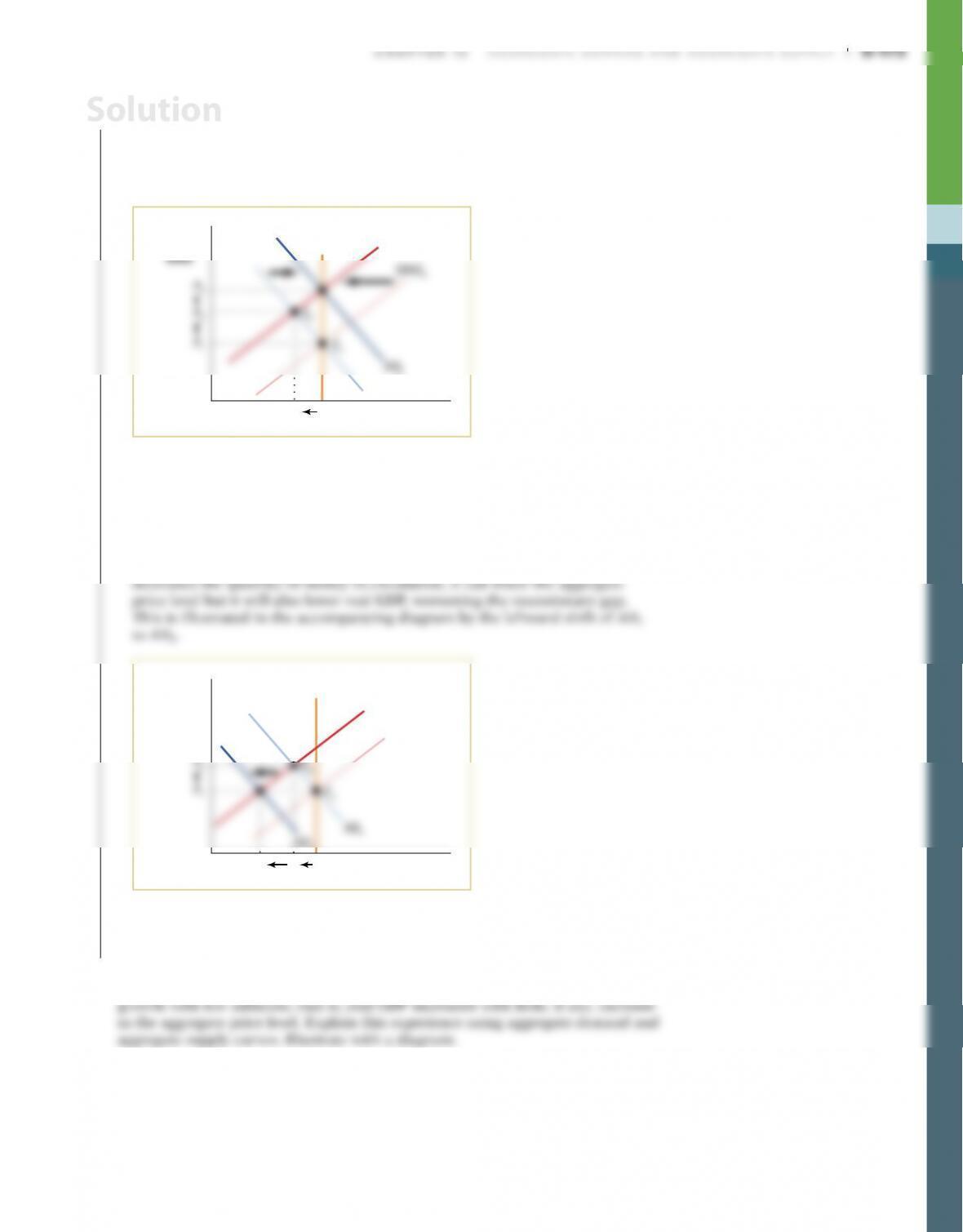
b. The government can use fiscal and monetary policies to either increase

real GDP or lower the aggregate price level, but not both. If the government

increases government spending, decreases taxes, or increases the quantity of

money in circulation, it can raise real GDP but it will also raise the aggregate

price level. This is illustrated in the diagram accompanying part a by the

rightward shift of AD1 to AD2.

If the government decreases government spending, increases taxes, or

Aggregate

price

level

Real GDPY2

LRAS

SRAS1

AD3

SRAS2

c. The government cannot use fiscal and monetary policies to correct for the

lower real GDP and higher aggregate price level simultaneously. It can only use

policies to alleviate one problem but at the expense of making the other worse.

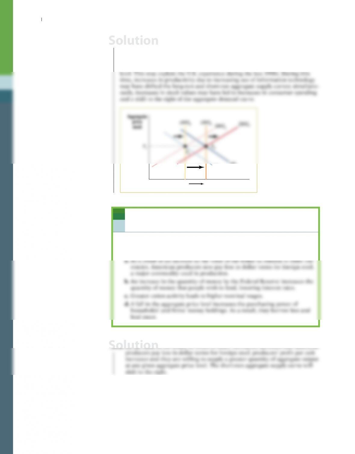
15. The late 1990s in the United States were characterized by substantial economic

Solution

S-174 Chapter 12 AggregAte DemAnD AnD AggregAte Supply

15. Increases in both long–run and short-run aggregate supply, along with increases

in aggregate demand, can explain how real GDP grew with little if any increase

in the aggregate price level. The accompanying diagram shows how the economy

could move from one long–run macroeconomic equilibrium, point E1, to another,

point E2, with an increase in real GDP and no increase in the aggregate price

Solution