
Chapter 12: Cash Flow Estimation and Risk Analysis
Learning Objectives
321
Chapter 12
Cash Flow Estimation and Risk Analysis
Learning Objectives
After reading this chapter, students should be able to do the following:
◆ Identify “relevant” cash flows that should and should not be included in a capital budgeting analysis.
◆ Estimate a project’s relevant cash flows and put them into a time line format that can be used to
calculate a project’s NPV, IRR, and other capital budgeting metrics.
◆ Explain how risk is measured, and use this measure to adjust the firm’s WACC to account for
differential project riskiness.
◆ Discuss how some projects can be altered after they have been accepted and how these alterations
can change a project’s cash flows and thus its realized NPV.
◆ Describe the post-audit, which is an important part of the capital budgeting process and discuss its
relevance in capital budgeting decisions.

322
Lecture Suggestions
Chapter 12: Cash Flow Estimation and Risk Analysis
Lecture Suggestions
This chapter covers some important but relatively technical topics. Note too that this chapter is more
modular than most, i.e., the major sections are discrete, hence they can be omitted without loss of
continuity. Therefore, if you are experiencing a time crunch, you could skip sections of the chapter.
What we cover, and the way we cover it, can be seen by scanning the slides and Integrated Case
solution for Chapter 12, which appears at the end of this chapter’s solutions. For other suggestions about the
lecture, please see the “Lecture Suggestions” in Chapter 2, where we describe how we conduct our classes.
DAYS ON CHAPTER: 5 OF 56 DAYS (50-minute periods)
Answers to End-of-Chapter Questions
12-1 Only cash can be spent or reinvested, and since accounting profits do not represent cash, they
12-2 Capital budgeting analysis should only include those cash flows that will be affected by the
decision. Sunk costs are unrecoverable and cannot be changed, so they have no bearing on the
12-3 When a firm takes on a new capital budgeting project, it typically must increase its investment in
receivables and inventories, over and above the increase in payables and accruals, thus
12-4 The costs associated with financing are reflected in the weighted average cost of capital. To
12-5 Daily cash flows would be theoretically best, but they would be costly to estimate and probably
no more accurate than annual estimates because we simply cannot forecast accurately at a daily
12-6 In replacement projects, the benefits are generally cost savings, although the new machinery
may also permit additional output. The data for replacement analysis are generally easier to
12-7 Stand-alone risk is the project’s risk if it is held as a lone asset. It disregards the fact that it is
but one asset within the firm’s portfolio of assets and that the firm is but one stock in a typical
investor’s portfolio of stocks. Stand–alone risk is measured by the variability of the project’s
12-8 It is often difficult to quantify market risk. On the other hand, we can usually get a good idea of
a project’s stand-alone risk, and that risk is normally correlated with market risk: The higher the
12-9 Simulation analysis involves working with continuous probability distributions, and the output of a
simulation analysis is a distribution of net present values or rates of return. Scenario analysis
12–10 Scenario analyses, and especially simulation analyses, would probably be reserved for very
important “make–or–break” decisions. They would not be used for every project decision because
12-11 The post-audit is a comparison of actual versus expected results for a given capital project. The
post-audit has two main purposes: (1) improve forecasts and (2) improve operations.
The post–audit is not a simple, mechanical process. First, we must recognize that each element
of the cash flow forecast is subject to uncertainty, so a percentage of all projects undertaken by any
Solutions to End-of-Chapter Problems
12-1 a. After-tax cost of equipment ($13,500,000)
NOWC investment (2,000,000)
12-2 a. Project cash flows: t = 1
Sales revenues $15,000,000
Operating costs 13,500,000
Depreciation: 100% Bonus taken at t = 0 0
12-3 Equipment’s original cost $29,000,000
Depreciation (100%) 29,000,000
326
Answers and Solutions
Chapter 12: Cash Flow Estimation and Risk Analysis
12-4 Cash outflow = $45,000.
Place the cash flows on a time line:
0 1 2 10
| | | • • • |
-45,000 8,000 8,000 8,000
12-6 a. The applicable depreciation values are as follows for the two scenarios:
Scenario 1 Scenario 2
Year (Straight-Line) (Bonus Deprec.)
0 $ 0 $800,000
1 200,000 0
b. To find the difference in net present values under these two methods, we must determine the
difference in incremental cash flows each method provides. The depreciation expenses cannot
simply be subtracted from each other, as there are tax ramifications due to depreciation
expense. The full depreciation expense is subtracted from revenues to arrive at operating
income (EBIT), and then taxes due are calculated. Then, depreciation is added to after-tax
Depreciation T × Depreciation
Year Expense (2 – 1) Expense
0 $800,000 $200,000
10%
Chapter 12: Cash Flow Estimation and Risk Analysis
Answers and Solutions
327
12-7 E(NPV) = 0.05(-$70) + 0.20(-$25) + 0.50($12) + 0.20($20) + 0.05($30)
= -$3.5 + -$5.0 + $6.0 + $4.0 + $1.5
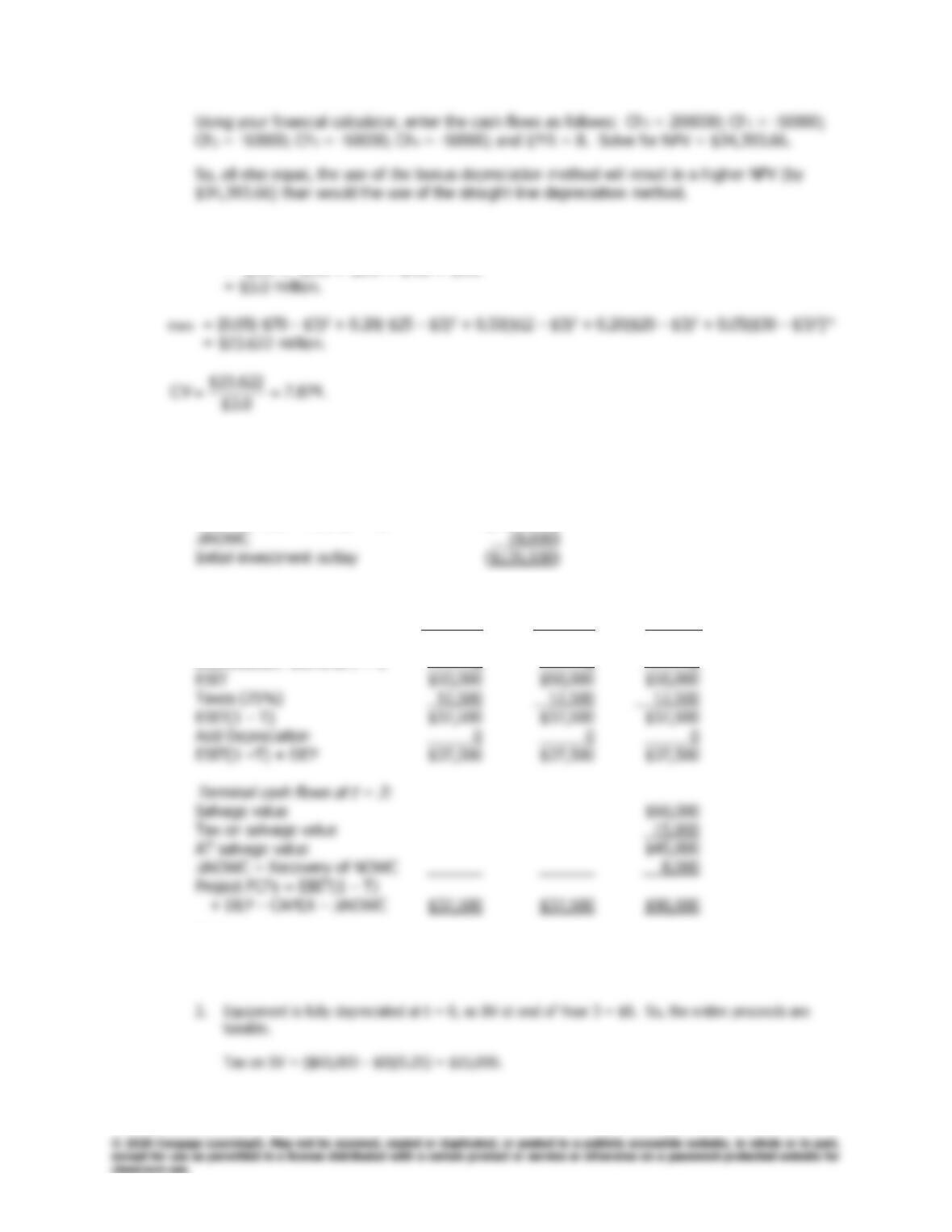
12-8 a. CF0 = –$135,500:
Initial investment outlay at t = 0:
After-tax cost = Cost (1 – T) ($127,500)
b.
Project’s operating cash flows:
Year 1 Year 2 Year 3
Savings $50,000 $50,000 $50,000
Depreciation: 100% at t = 0 0 0 0
Notes:
1. Equipment is immediately expensed in Year 0, so there is no depreciation expense in Years 1, 2, and
3.
328
Answers and Solutions
Chapter 12: Cash Flow Estimation and Risk Analysis
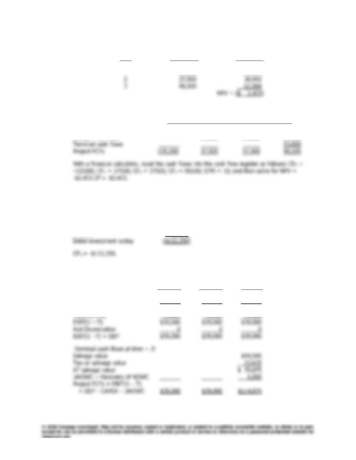
c. The project has an NPV of ($2,423). Thus, it should not be accepted.
Year Cash Flows PV @ 10%
0 ($135,500) ($135,500)
1 37,500 34,091
Alternatively, place the free cash flows on a time line:
0 1 2 3
| | | |
Initial investment outlay -135,500
EBIT(1 – T) + DEP 37,500 37,500 37,500
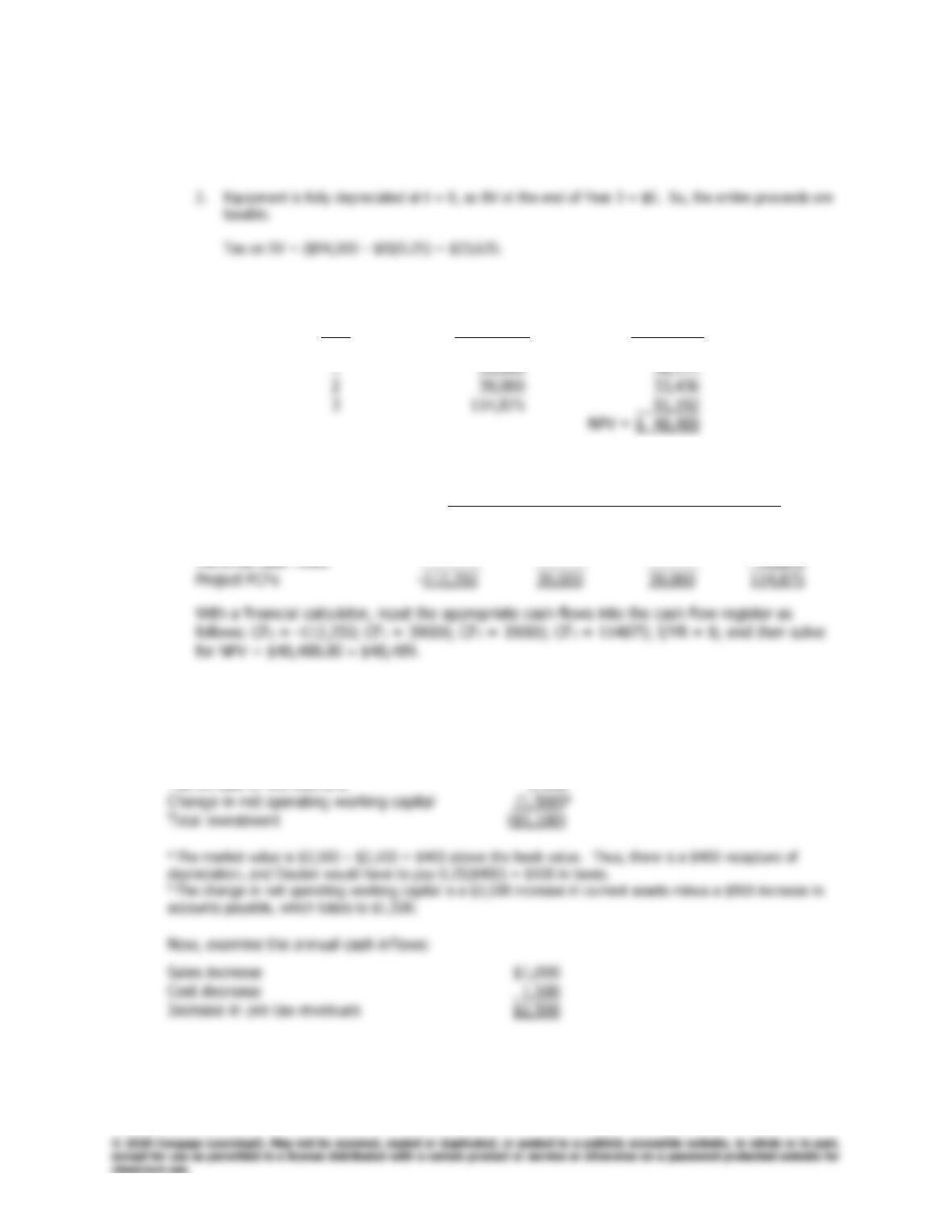
12-9 a. The $4,500 spent last year on exploring the feasibility of the project is a sunk cost and should
not be included in the analysis.
b. The initial investment outlay at t = 0 is $112,250:
CAPEX = Cost (1 – T) ($107,250)
NOWC (5,000)
c. The annual project cash flows follow:
Project’s operating cash flows:
Year 1 Year 2 Year 3
Savings $52,000 $52,000 $52,000
Depreciation: 100% at t = 0 0 0 0
EBIT $52,000 $52,000 $52,000
10%
Chapter 12: Cash Flow Estimation and Risk Analysis
Answers and Solutions
329
Notes:
1. Equipment is immediately expensed in Year 0, so there is no depreciation expense in Years 1, 2, and
3.
d. The project has an NPV of $48,489; thus, it should be accepted.
Year Cash Flows PV @ 8%
0 ($112,250) ($112,250)
Alternatively, place the free cash flows on a time line:
0 1 2 3
| | | |
Initial investment outlay -112,250
EBIT(1 – T) + DEP 39,000 39,000 39,000
12–10 First determine the net cash flow at t = 0:
After-tax cost of new equipment ($6,000)
Sale of old machine 2,500
Tax on sale of old machine (100)a
8%
330
Answers and Solutions
Chapter 12: Cash Flow Estimation and Risk Analysis
After-tax revenue increase:
$2,500(1 – T) = $2,500(0.75) = $1,875.
Depreciation:
Year 1 2 3 4 5 6
Newa $ 0 $ 0 $ 0 $ 0 $ 0 $ 0
Old 350 350 350 350 350 350
Now recognize that at the end of Year 6 Dauten would recover its net operating working capital
investment of $1,500, and it would also receive $800 from the sale of the replacement machine.
However, since the machine would be fully depreciated, the firm must pay 0.25($800) = $200 in
Finally, place all the cash flows on a time line:
0 1 2 3 4 5 6
| | | | | | |
Net investment (5,100)
After-tax revenue increase 1,875 1,875 1,875 1,875 1,875 1,875
12-11 1. Net investment at t = 0:
11%
Chapter 12: Cash Flow Estimation and Risk Analysis
Answers and Solutions
331
2. After–tax Increase
Year in Earnings T(Dep) Annual CFt
1 $16,500 $ 0 $16,500
2 16,500 0 16,500
3 16,500 0 16,500
Notes:
a. The after-tax increase in earnings are $22,000(1 – T) = $22,000(0.75) = $16,500.
3. Now find the NPV of the replacement machine:
Place the cash flows on a time line:
0 1 2 3 4 5 6 7 8
| | | | | | | | |
-60,000 16,500 16,500 16,500 16,500 16,500 16,500 16,500 16,500
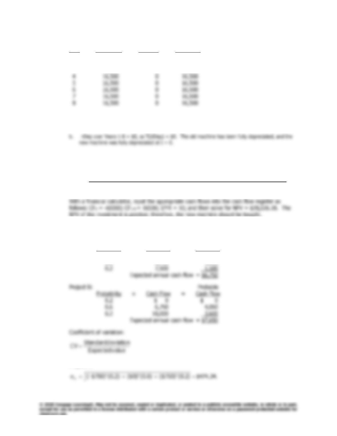
12–12 a. Expected annual cash flows:
Project A: Probable
Probability × Cash Flow = Cash Flow
0.2 $6,000 $1,200
0.6 6,750 4,050
Project A:
10%
332
Answers and Solutions
Chapter 12: Cash Flow Estimation and Risk Analysis
Project B:
b. Project B is the riskier project because it has the greater variability in its probable cash flows,
whether measured by the standard deviation or the coefficient of variation. Hence, Project B is
evaluated at the 12% cost of capital, while Project A requires only a 10% cost of capital.
c. The portfolio effects from Project B would tend to make it less risky than otherwise. This would
tend to reinforce the decision to accept Project B. Again, if Project B were negatively
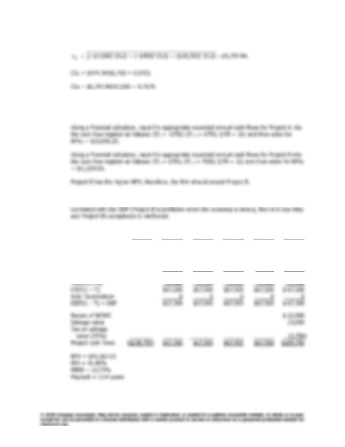
12-13 a. 0 1 2 3 4 5
Capex (1 – T) ($213,750)
NOWC (25,000)
Cost savings $90,000 $90,000 $90,000 $90,000 $ 90,000
Depreciationa 0 0 0 0 0
EBIT $90,000 $90,000 $90,000 $90,000 $ 90,000
Chapter 12: Cash Flow Estimation and Risk Analysis
Answers and Solutions
333
Notes:
a The new machine qualifies for immediate expensing (bonus depreciation), so it is fully depreciated at t =
0. Therefore, annual depreciation in Years 1 through 5 is zero.
b. If savings increase by 20%, then savings will be (1.2)($90,000) = $108,000.
(1) Savings increase by 20%:
0 1 2 3 4 5
Capex (1 – T) ($213,750)
NOWC (25,000)
Cost savings $108,000 $108,000 $108,000 $108,000 $108,000
Depreciation 0 0 0 0 0
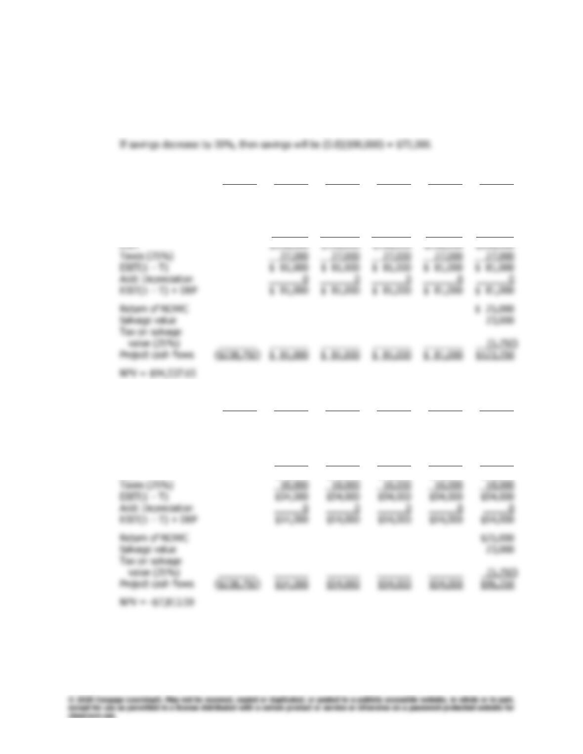
(2) Savings decrease by 20%:
0 1 2 3 4 5
Capex (1 – T) ($213,750)
NOWC (25,000)
Cost savings $72,000 $72,000 $72,000 $72,000 $72,000
Depreciation 0 0 0 0 0
EBIT $72,000 $72,000 $72,000 $72,000 $72,000
334
Answers and Solutions
Chapter 12: Cash Flow Estimation and Risk Analysis
c. Worst-case scenario:
0 1 2 3 4 5
Capex (1 – T) ($213,750)
NOWC (30,000)
Cost savings $72,000 $72,000 $72,000 $72,000 $72,000
Depreciation 0 0 0 0 0
EBIT $72,000 $72,000 $72,000 $72,000 $72,000
Return of NOWC $30,000
Salvage value 18,000
Tax on salvage
Base-case scenario:
Best-case scenario:
0 1 2 3 4 5
Capex (1 – T) ($213,750)
NOWC (20,000)
Cost savings $108,000 $108,000 $108,000 $108,000 $108,000
Depreciation 0 0 0 0 0
EBIT $108,000 $108,000 $108,000 $108,000 $108,000
Return of NOWC $ 20,000
Salvage value 28,000
Tax on salvage
NPV = $98,761.50
Prob. NPV Prob. NPV
Worst-case 0.35 ($12,037.44) ($ 4,213.10)
Chapter 12: Cash Flow Estimation and Risk Analysis
Answers and Solutions
335
NPV = [(0.35)(-$12,037.44 – $40,592.06)2 + (0.35)($43,362.03 – $40,592.06)2 +
(0.30)($98,761.50 – $40,592.06)2]½
12–14 a. Old depreciation = $8,500 per year.
Book value = $85,000 – 5($8,500) = $42,500.
Gain = $55,000 – $42,500 = $12,500.
b. The new machine is eligible for 100% bonus depreciation, so there is no annual depreciation for
the new machine.
Depreciation Depreciation Change in
Year Allowance, New Allowance, Old Depreciation
1 $0 $8,500 ($8,500)
CFt = (Operating expenses)(1 – T) + (Depreciation)(T).
CF1 = ($40,000)(0.75) − ($8,500)(0.25) = $30,000 − $2,125 = $27,875.
CF2 = ($40,000)(0.75) − ($8,500)(0.25) = $30,000 − $2,125 = $27,875.
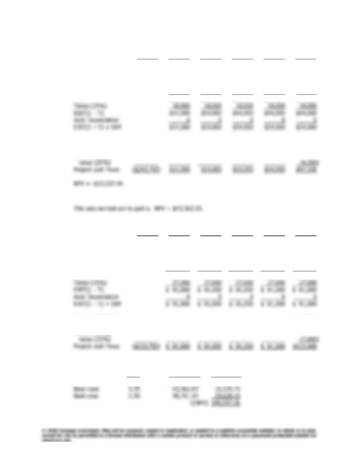
0 1 2 3 4 5
| | | | | |
Capex (1 – T) (75,625)
Operating CFs 27,875 27,875 27,875 27,875 27,875
c. From part b input the data into your calculator as follows: CF0 = -75625; CF1 = 27875; CF2 =
9%
336
Answers and Solutions
Chapter 12: Cash Flow Estimation and Risk Analysis
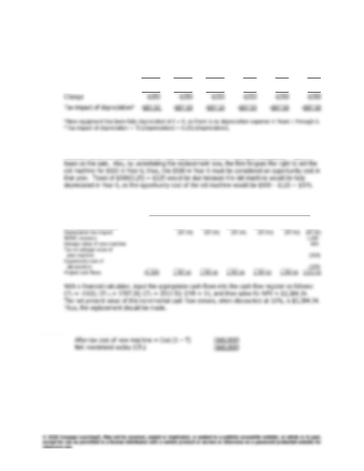
12–15 a. After-tax cost of new machine ($881,250)
b. The new machine is eligible for 100% bonus depreciation, so there is no annual depreciation
for the new machine.
Depreciation Depreciation Change in
Year Allowance, New Allowance, Old Depreciation
1 $0 $120,000 ($120,000)
c. CFt = (Operating expenses)(1 – T) + (Depreciation)(T).
CF1 = ($220,000)(0.75) − ($120,000)(0.25) = $165,000 − $30,000 = $135,000.
CF2 = ($220,000)(0.75) − ($120,000)(0.25) = $165,000 − $30,000 = $135,000.
A time line of the cash flows looks like this:
0 1 2 3 4 5
| | | | | |
(532,500) 135,000 135,000 135,000 135,000 135,000
*After-tax salvage value of new machine at Year 5. Since the machine is fully depreciated at t = 0, the
book value is zero. After-tax salvage value is calculated as follows:
d. From part c input the data into your calculator as follows: CF0 = –532500; CF1 = 135000; CF2
12%
Chapter 12: Cash Flow Estimation and Risk Analysis
Answers and Solutions
337
e. 1. If the expected life of the old machine decreases, the new machine will look better as cash
12-16 a. NPV of abandonment after Year t:
Using a financial calculator, input the following: CF0 = -22500, CF1 = 22875, and I/YR = 9 to
solve for NPV1 = -$1,513.76 -$1,514.
Using a financial calculator, input the following: CF0 = -22500, CF1 = 5875, CF2 = 20875, and
12-17 a. WACC = 12.5%.
Since each project is independent and of average risk, all projects whose IRR > WACC will be
accepted. Consequently, Projects A, B, C, D, and E will be accepted, and the optimal capital
budget is $5,250,000.
338
Comprehensive/Spreadsheet Problem
Chapter 12: Cash Flow Estimation and Risk Analysis
Comprehensive/Spreadsheet Problem
Note to Instructors:
The solution to this problem is not provided to students at the back of their text. Instructors
can access the
Excel
file on the textbook’s website.
12–18 a.
Net Present Value (at 10% ) $20,507
Data for Payback Years 0 1 2 3
Cumulative CF from Row 63 (151,250) (91,625) (32,000) 58,875
b. The $30,000 R&D costs are sunk costs. Therefore, these costs will have no effect on NPV and
other profitability measures.
c. If the new project will reduce cash flows from the firm’s other projects, then this is a negative
externality and must be considered in the analysis. Consequently, these should be considered
Chapter 12: Cash Flow Estimation and Risk Analysis
Comprehensive/Spreadsheet Problem
339
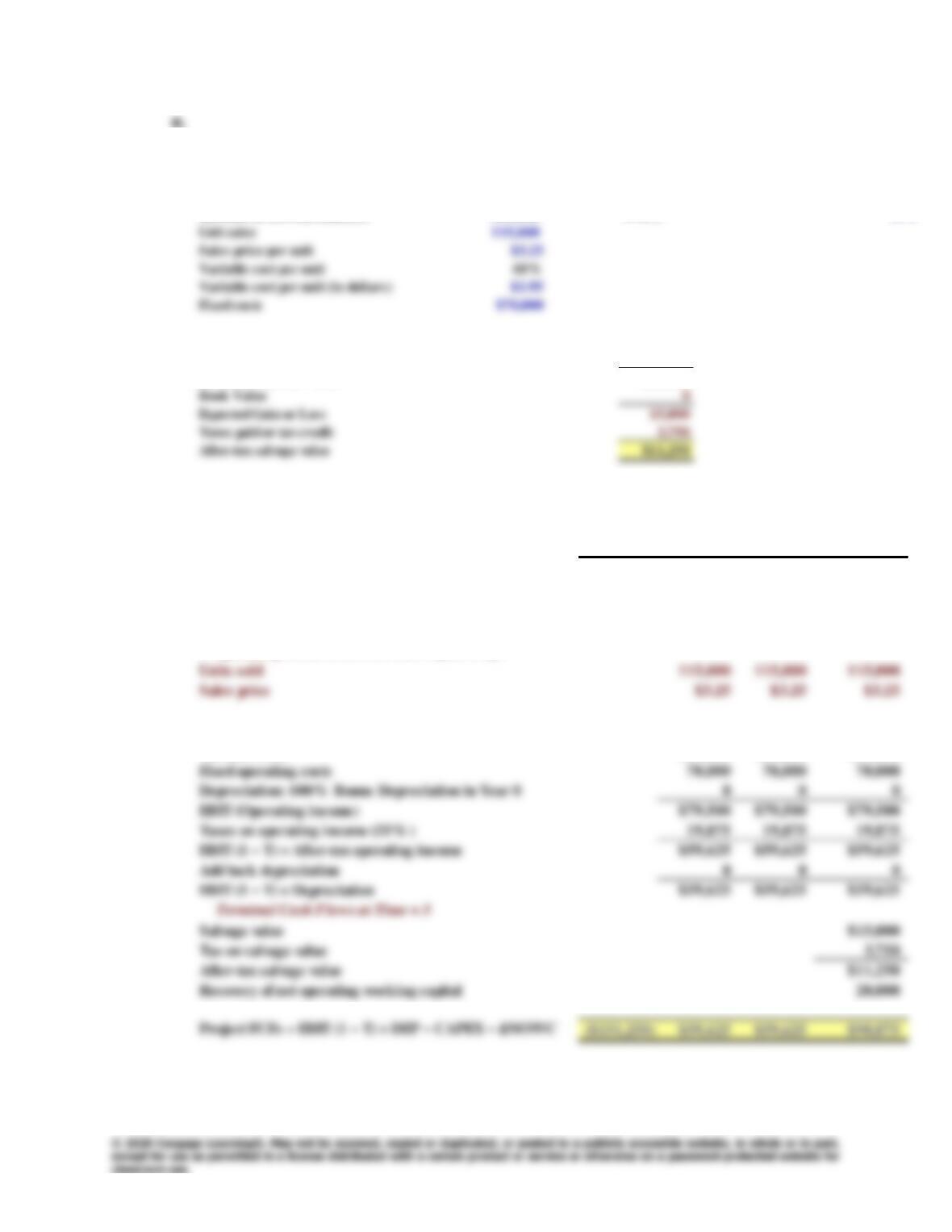
Part 1. Key Input Data
Equipment cost plus installation $175,000 Market value of equipment after 3 yrs $15,000
Increase in current assets $35,000 Tax rate 25%
Increase in current liabilities $15,000 WACC 10%
Part 2. After-Tax Salvage Value at end of Year 3 Equipment
Estimated Market Value $15,000
Part 3. Project Cash Flow Analysis
0 1 2 3
Investment Outlays at Time = 0
CAPEX = Equipment = Cost (1 − T) (131,250)
Increase in NOWC (20,000)
Operating Cash Flows over the Project‘s Life
Sales revenues $373,750 $373,750 $373,750
Variable costs 224,250 224,250 224,250
Part 4. Key Output: Evaluation of the Proposed Project
Net Present Value (at 10% ) $20,507
IRR 17.00%
Data for Payback Years 0 1 2 3
Cumulative CF from Row 63 (151,250) (91,625) (32,000) 58,875
f.
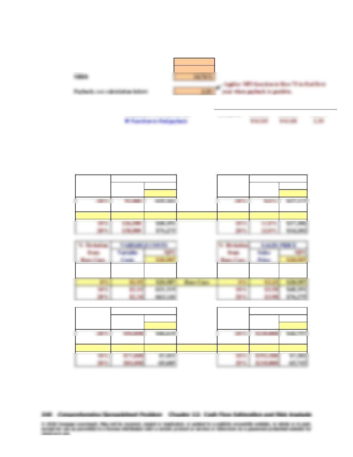
Sensitivity of NPV to Changes in Inputs. Here we use an Excel “Data Table” to find NPV
if each variable were better or worse than the base-case level, holding other things constant.
% Deviation % Deviation
from Units NPV from NPV
Base Case Sales $20,507 Base Case WACC 20,507
–10% 103,500 –$7,377 –10% 9.0% $23,809
0% 115,000 $20,507 Base Case 0% 10.0% $20,507
–20% $1.56 $104,159 –20% $2.60 –$35,261
–10% $1.76 $62,333 –10% $2.93 –$7,377
% Deviation % Deviation
from Fixed NPV from Equipment NPV
Base Case Costs $20,507 Base Case Cost $20,507
–10% $63,000 $33,563 –10% $157,500 $33,632
0% $70,000 $20,507 Base Case 0% $175,000 $20,507
WACC
UNIT SALES
FIXED COSTS
EQUIPMENT COST