12 Case model 12/09/2018
Allied Food Products is considering expanding into the fruit juice business with a new fresh
lemon juice product. Assume that you were recently hired as assistant to the director of capital
budgeting and you must evaluate the new project.
The project is expected to operate for 4 years, at which time it will be terminated. The cash
inflows are assumed to begin 1 year after the project is undertaken, or at t = 1, and to continue
out to t = 4. At the end of the project’s life (t = 4), the equipment is expected to have a salvage
value of $25,000.
Unit sales are expected to total 100,000 units per year, and the expected sales price is $2.00 per
unit. Cash operating costs for the project are expected to total 60% of dollar sales. Allied’s tax rate
is 25%, and its WACC is 10%. Tentatively, the lemon juice project is assumed to be of equal risk to
Allied’s other assets.
You have been asked to evaluate the project and to make a recommendation as to whether it
should be accepted or rejected. To guide you in your analysis, your boss gave you the following
set of tasks/questions.
INPUT DATA
Initial Costs
Equipment $280,000
Expected salvage value $25,000
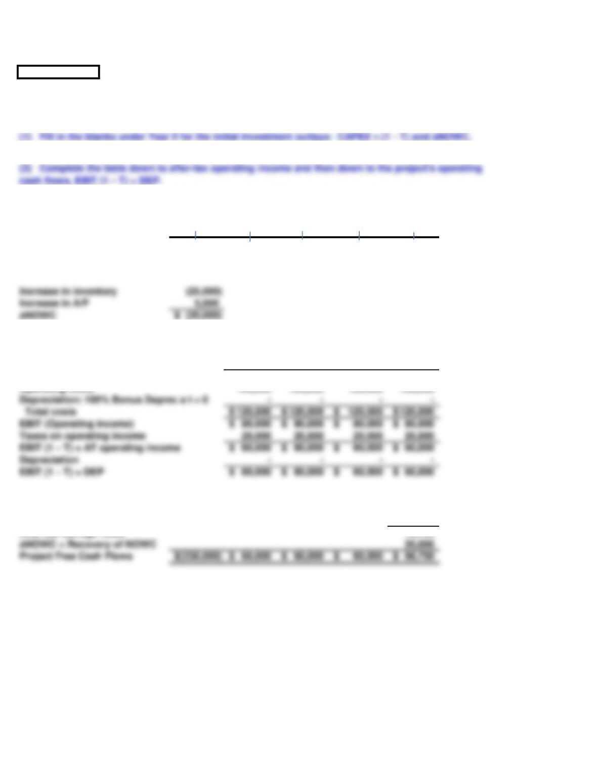
Changes in NOWC
Inventories $25,000
Accounts payable $5,000
Expected unit sales 100,000
Price per unit $2.00
Oper. costs (% of sales) 60.0%
Tax rate 25.0%
9/12/2022 17:20
Chapter 12. Cash Flow Estimation and Risk Analysis
This spreadsheet model is designed to be used in conjunction with the chapter’s
integrated case and the related PowerPoint slide presentation.
Allied owns the building, which is fully depreciated. The purchase price of the required equipment
depreciation at the time of purchase. In addition, inventories would rise by $25,000, while accounts
payable would increase by $5,000. All of these costs would be incurred at t = 0.
PART A
Allied has a standard form that is used in the capital budgeting process; see Table IC12.1. Part
of the table has been completed, but you must replace the blanks with the missing numbers.
Complete the table in the following steps:
Years
0 1 2 3 4
I. Investment Outlays
CAPEX × (1 − T) (210,000)$
Increase in inventory (25,000)
Increase in A/P 5,000
II. Project Operating Cash Flows
Unit sales 100,000 100,000 100,000 100,000
Price per unit 2.00$ 2.00$ 2.00$ 2.00$
Total revenues 200,000$ 200,000$ 200,000$ 200,000$
Operating costs 120,000 120,000 120,000 120,000
Depreciation: 100% Bonus Deprec a t = 0 – – – –
Total costs 120,000$ 120,000$ 120,000$ 120,000$
EBIT (Operating income) 80,000$ 80,000$ 80,000$ 80,000$
Taxes on operating income 20,000 20,000 20,000 20,000
EBIT (1 ‒ T) = AT operating income 60,000$ 60,000$ 60,000$ 60,000$
EBIT (1 ‒ T) + DEP 60,000$ 60,000$ 60,000$ 60,000$
III. Project Termination Cash Flows
Salvage value 25,000
Tax on salvage value (6,250)
After-tax salvage value 18,750
(4) Fill in the blanks under Year 4 for the terminal cash flows, and complete the project
free cash flow line.
(3) Complete the table down to after-tax operating income and then down to the project’s operating
cash flows, EBIT (1 ‒ T) + DEP.
(2) Complete the table for unit sales, sales price, total revenues, and operating costs.
(1) Fill in the blanks under Year 0 for the initial investment outlays: CAPEX × (1 − T) and ΔNOWC.
PART C
Disregard all the assumptions made in part B, and assume there is no alternative use for the
building over the next 4 years. Now calculate the project’s NPV, IRR, MIRR, and payback. Do
these indicators suggest that the project should be accepted? Explain.
The decision criteria introduced in Chapter 11 are used to evaluate this project.
IV. Results
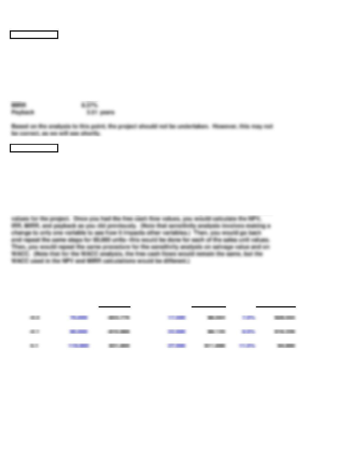
NPV -$13,341
IRR 7.50%
PART F
(2) How would you perform a sensitivity analysis on the unit sales, salvage value, and WACC
for the project? Assume that each of these variables deviates from its base-case, or
expected, value by plus or minus 10%, 20%, and 30%.
The base-case value for unit sales was 100,000; therefore, if you were to assume that this value
deviated by plus and minus 10%, 20%, and 30%, the unit sales values to be used in the sensitivity
analysis would be 70,000, 80,000, 90,000, 110,000, 120,000, and 130,000 units. You would then go
back to the table at the beginning of the problem, insert the appropriate sales unit number, say
70,000 units, and rework the table for the change in sales units arriving at different free cash flow
values for the project. Once you had the free cash flow values, you would calculate the NPV,
IRR, MIRR, and payback as you did previously. (Note that sensitivity analysis involves making a
change to only one variable to see how it impacts other variables.) Then, you would go back
and repeat the same steps for 80,000 units–this would be done for each of the sales unit values.
Then, you would repeat the same procedure for the sensitivity analysis on salvage value and on
WACC. (Note that for the WACC analysis, the free cash flows would remain the same, but the
WACC used in the NPV and MIRR calculations would be different.)
Excel is ideally suited for sensitivity analysis. Using data tables, the sensitivity analysis is simple.
SENSITIVITY ANALYSIS DATA TABLES
Unit Sales
Salvage
Value
WACC
$10,406 $10,406 $10,406
-0.3 70,000 -$53,776 17,500 $6,564 7.0% $28,555
-0.2 80,000 -$32,382 20,000 $7,844 8.0% $22,272
-0.1 90,000 -$10,988 22,500 $9,125 9.0% $16,226
0.0 100,000 $10,406 25,000 $10,406 10.0% $10,406
0.1 110,000 $31,800 27,500 $11,686 11.0% $4,800
0.2 120,000 $53,194 30,000 $12,967 12.0% -$602
0.3 130,000 $74,588 32,500 $14,248 13.0% -$5,809
Based on the analysis to this point, the project should not be undertaken. However, this may not
be correct, as we will see shortly.
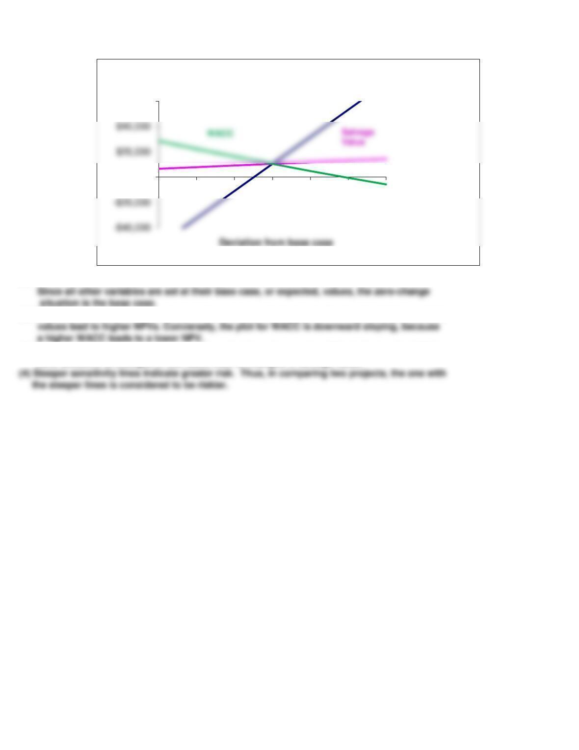
(1) The sensitivity lines intersect at 0% change and the base-case NPV, at $10,406.
(2) The plots for unit sales and salvage value are upward sloping, indicating that higher variable
(3) The plot of unit sales is much steeper than that for salvage value. This indicates that NPV is
more sensitive to changes in unit sales than to changes in salvage value.
(4) Steeper sensitivity lines indicate greater risk. Thus, in comparing two projects, the one with
the steeper lines is considered to be riskier.
$0
$60,000
-30% -20% -10% 0% 10% 20% 30%
NPV
Sensitivity analysis
Unit
Sales
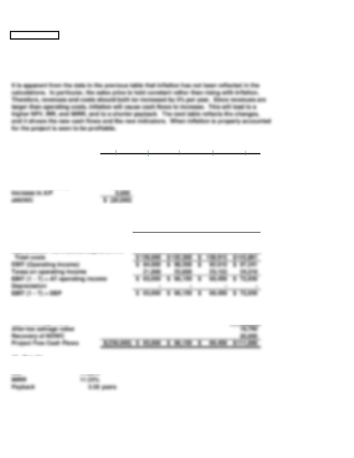
PART G
Assume that inflation is expected to average 5% over the next 4 years, and that this expectation is
reflected in the WACC. Moreover, inflation is expected to increase revenues and variable costs
by this same 5%. Does it appear that inflation has been dealt with properly in the initial analysis
to this point? If not, what should be done, and how would the required adjustment affect the
decision?
Expected inflation 5%
Years
0 1 2 3 4
I. Investment Outlays
CAPEX × (1 − T) (210,000)$
Increase in inventory (25,000)
Increase in A/P 5,000
II. Project Operating Cash Flows
Unit sales 100,000 100,000 100,000 100,000
Price per unit 2.10$ 2.21$ 2.32$ 2.43$
Total revenues 210,000 220,500 231,525 243,101
Operating costs 126,000 132,300 138,915 145,861
Depreciation: 100% Bonus Deprec a t = 0 – – – –
Total costs 126,000$ 132,300$ 138,915$ 145,861$
EBIT (Operating income) 84,000$ 88,200$ 92,610$ 97,241$
Taxes on operating income 21,000 22,050 23,153 24,310
EBIT (1 ‒ T) = AT operating income 63,000$ 66,150$ 69,458$ 72,930$
EBIT (1 ‒ T) + DEP 63,000$ 66,150$ 69,458$ 72,930$
III. Terminal Year Cash Flows
Salvage value 25,000
Tax on salvage value (6,250)
After-tax salvage value 18,750
Recovery of NOWC 20,000
IV. Results
NPV $10,406
It is apparent from the data in the previous table that inflation has not been reflected in the
calculations. In particular, the sales price is held constant rather than rising with inflation.
Therefore, revenues and costs should both be increased by 5% per year. Since revenues are
larger than operating costs, inflation will cause cash flows to increase. This will lead to a
higher NPV, IRR, and MIRR, and to a shorter payback. The next table reflects the changes,
and it shows the new cash flows and the new indicators. When inflation is properly accounted
for the project is seen to be profitable.
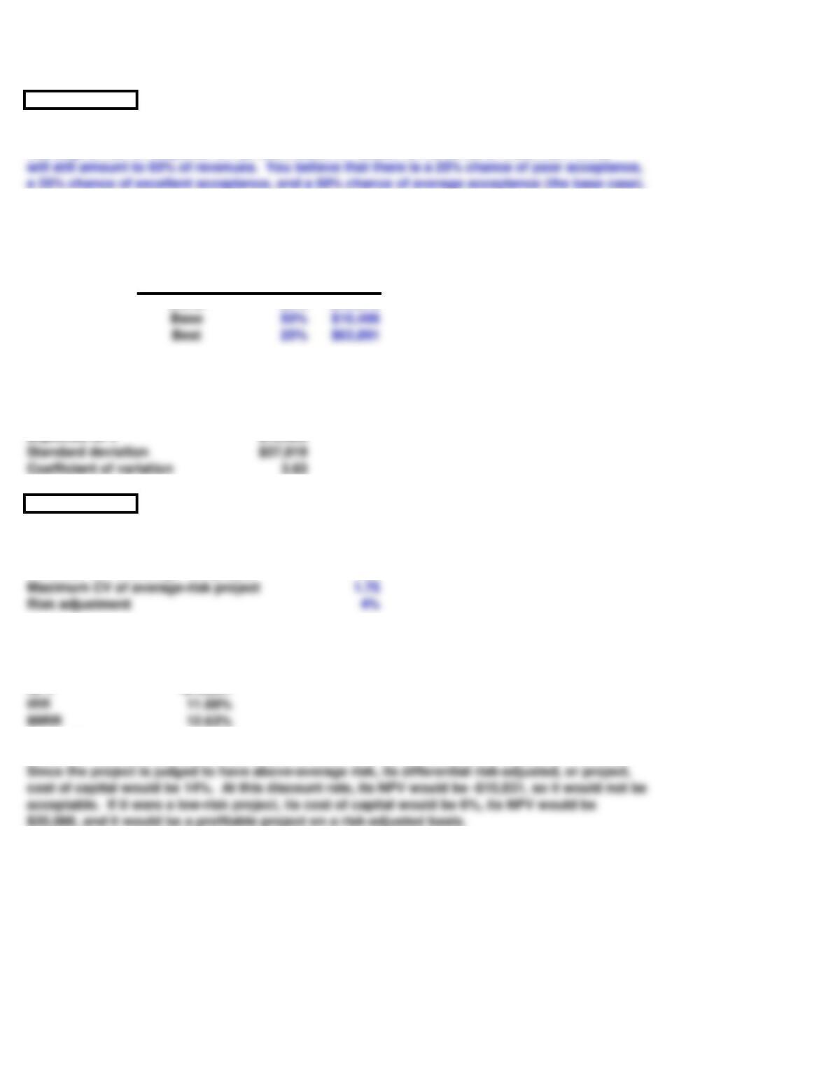
PART H
Assume that you are confident about the estimates of all the variables that affect the cash flows
except unit sales. If product acceptance is poor, sales will be only 75,000 units a year, while
a strong consumer response will produce sales of 125,000 units. In either case, cash costs
(1) What is the worst-case NPV? The best-case NPV?
We used this spreadsheet model to develop these scenarios:
Case Probability NPV
Worst 25% -$43,079
(2) Use the worst-case, most likely case (or base-case), and best-case NPVs with their
probabilities of occurrence to find the project’s expected NPV, standard
deviation, and coefficient of variation.
Expected NPV $10,406
Standard deviation $37,819
Coefficient of variation 3.63
PART M
Allied typically adds or subtracts 4% to its WACC to adjust for risk. After adjusting for risk, should
the lemon juice project be accepted?
Minimum CV of average-risk project 1.25
Maximum CV of average-risk project 1.75
Risk adjustment 4%
WACC 14%
Results
NPV -$10,831
Payback 3.28 years
Since the project is judged to have above-average risk, its differential risk-adjusted, or project,
cost of capital would be 14%. At this discount rate, its NPV would be -$10,831, so it would not be
acceptable. If it were a low-risk project, its cost of capital would be 6%, its NPV would be
will still amount to 60% of revenues. You believe that there is a 25% chance of poor acceptance,
a 25% chance of excellent acceptance, and a 50% chance of average acceptance (the base case).