Questions for Review
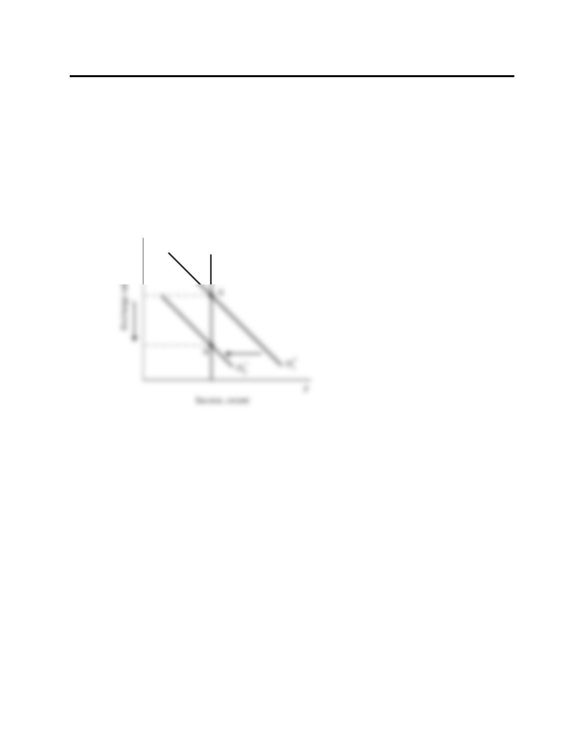
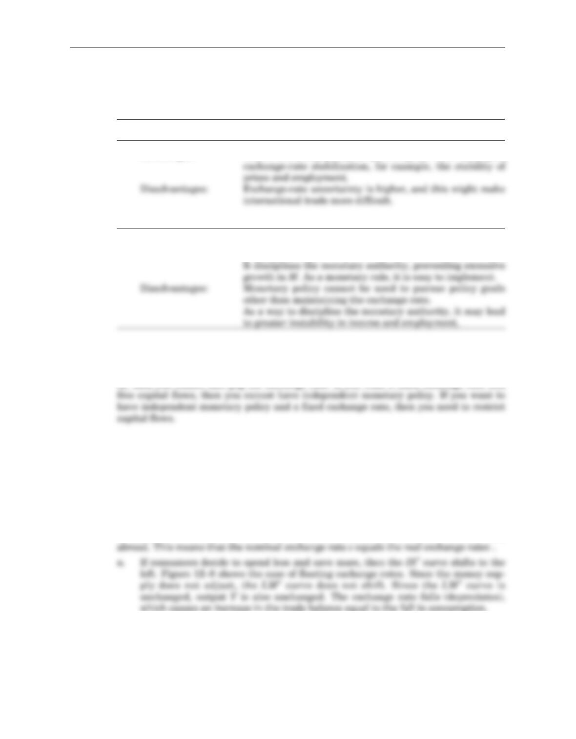
1. In the Mundell–Fleming model, an increase in taxes shifts the IS* curve to the left. If
the exchange rate floats freely, then the LM*curve is unaffected. As shown in Figure
12–1, the exchange rate falls while aggregate income remains unchanged. The fall in
the exchange rate causes the trade balance to increase.
119
e
LM*
Figure 12–1
CHAPTER 12 The Open Economy Revisited
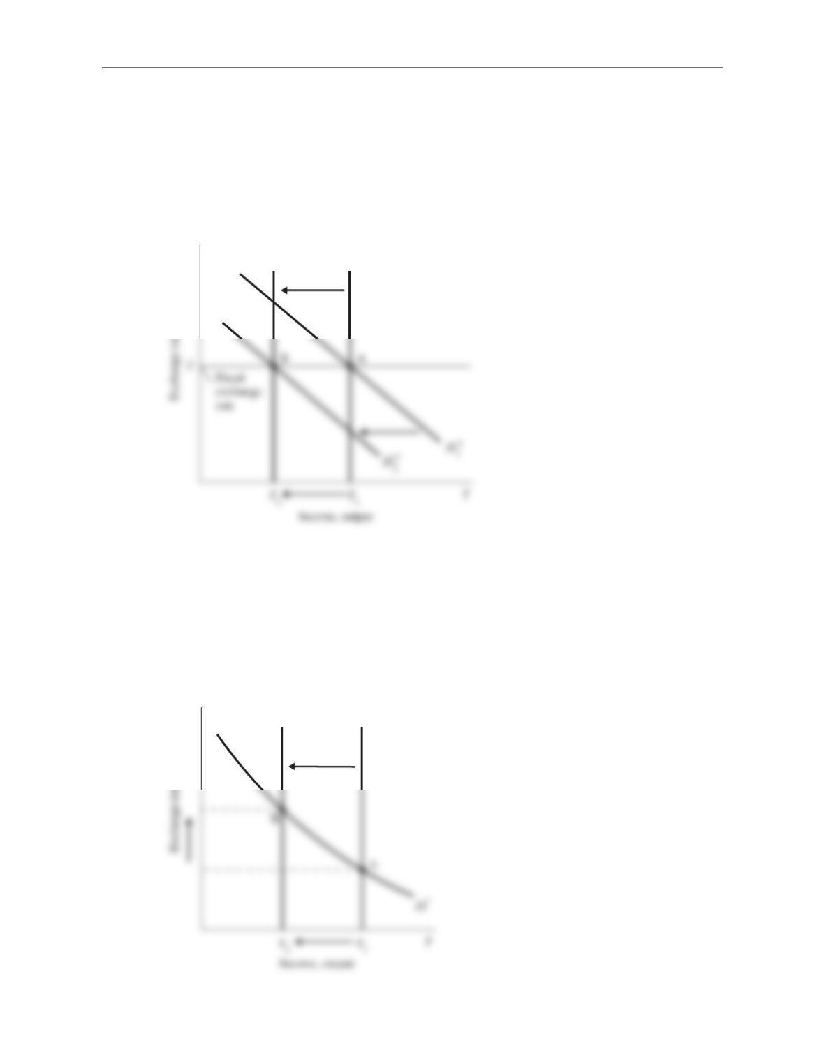
Now suppose there are fixed exchange rates. When the IS*curve shifts to the left
in Figure 12–2, the money supply has to fall to keep the exchange rate constant, shift-
ing the LM*curve from LM*
1to LM*
2. As shown in the figure, output falls while the
exchange rate remains fixed.
Net exports can only change if the exchange rate changes or the net exports sched-
ule shifts. Neither occurs here, so net exports do not change.
We conclude that in an open economy, fiscal policy is effective at influencing out-
put under fixed exchange rates but ineffective under floating exchange rates.
2. In the Mundell–Fleming model with floating exchange rates, a reduction in the money
supply reduces real balances M/P, causing the LM*curve to shift to the left. As shown
in Figure 12–3, this leads to a new equilibrium with lower income and a higher
exchange rate. The increase in the exchange rate reduces the trade balance.
120 Answers to Textbook Questions and Problems
e
LM2LM1
**
Figure 12–2
e
LM2LM1
** Figure 12–3
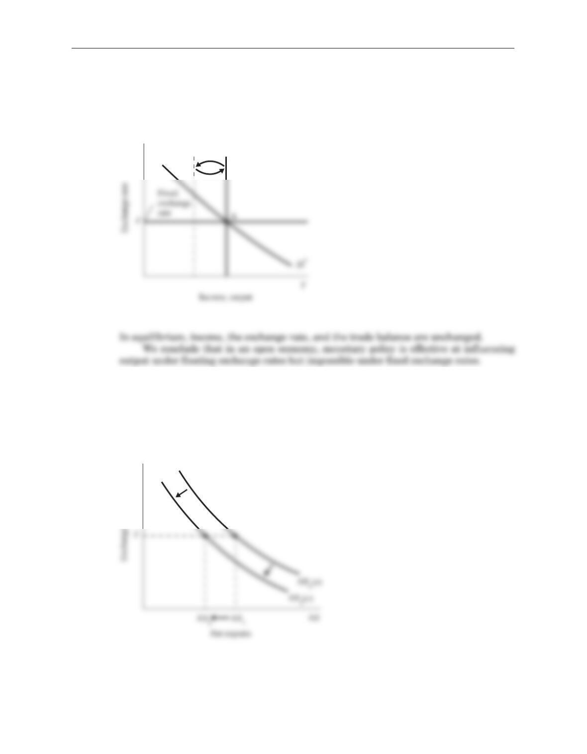
If exchange rates are fixed, then the upward pressure on the exchange rate forces
the Fed to sell dollars and buy foreign exchange. This increases the money supply M
and shifts the LM*curve back to the right until it reaches LM*
1again, as shown in
Figure 12–4.
3. In the Mundell–Fleming model under floating exchange rates, removing a quota on
imported cars shifts the net exports schedule inward, as shown in Figure 12–5. As in
the figure, for any given exchange rate, such as e, net exports fall. This is because it
now becomes possible for Americans to buy more Toyotas, Volkswagens, and other for-
eign cars than they could when there was a quota.
Chapter 12 Aggregate Demand in the Open Economy 121
e
LM1
*
Figure 12–4
e
Figure 12–5
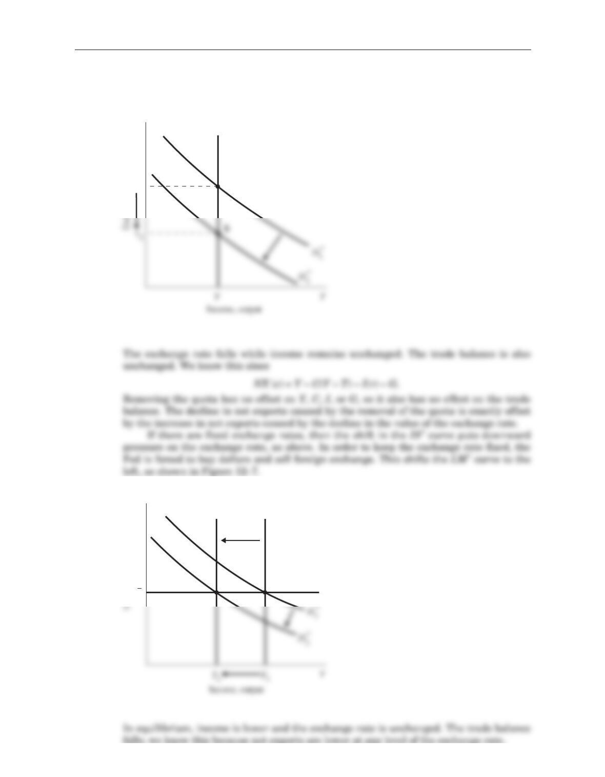
This inward shift in the net-exports schedule causes the IS*schedule to shift
inward as well, as shown in Figure 12–6.
122 Answers to Textbook Questions and Problems
e
A
e1
LM *
Figure 12–6
e
e
BA e
LM2LM1
**
Figure 12–7
4. The following table lists some of the advantages and disadvantages of floating versus
fixed exchange rates.
Table 12–1
Floating Exchange Rates
Advantages: Allows monetary policy to pursue goals other than just
Fixed Exchange Rates
Advantages: Makes international trade easier by reducing exchange
rate uncertainty.
5. The impossible trinity states that it is impossible for a nation to have free capital flows,
a fixed exchange rate, and independent monetary policy. In other words, you can only
have two of the three. If you want free capital flows and an independent monetary poli-
cy, then you cannot also peg the exchange rate. If you want a fixed exchange rate and
Problems and Applications
1. The following three equations describe the Mundell–Fleming model:
Y= C(Y– T) + I(r) + G+ NX(e). (IS)
M/P = L(r, Y). (LM)
r= r*.
In addition, we assume that the price level is fixed in the short run, both at home and
Chapter 12 Aggregate Demand in the Open Economy 123
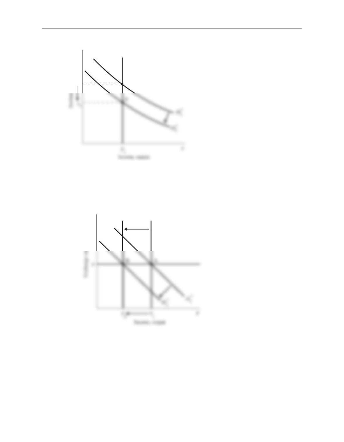
Figure 12–9 shows the case of fixed exchange rates. The IS*curve shifts to
the left, but the exchange rate cannot fall. Instead, output falls. Since the
exchange rate does not change, we know that the trade balance does not change
either.
In essence, the fall in desired spending puts downward pressure on the inter-
est rate and, hence, on the exchange rate. If there are fixed exchange rates, then
the central bank buys the domestic currency that investors seek to exchange, and
provides foreign currency, shifting LM* to the left. As a result, the exchange rate
does not change, so the trade balance does not change. Hence, there is nothing to
offset the fall in consumption, and output falls.
124 Answers to Textbook Questions and Problems
e
A
e1
LM *
Figure 12–8
e
LM2LM1
**
Figure 12–9
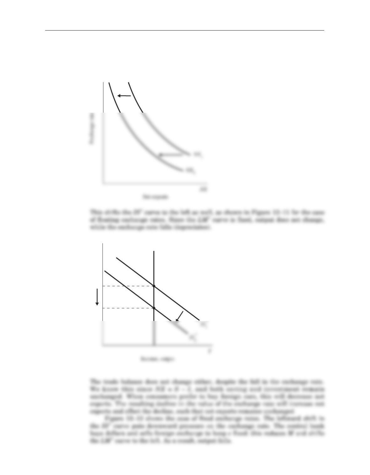
b. If some consumers decide they prefer stylish Toyotas to Fords and Chryslers, then
the net-exports schedule, shown in Figure 12–10, shifts to the left. That is, at any
level of the exchange rate, net exports are lower than they were before.
Chapter 12 Aggregate Demand in the Open Economy 125
e
Exchange rate
A
B
LM*
e1
e2
Figure 12–11
e
Figure 12–10
126 Answers to Textbook Questions and Problems
The trade balance falls, because the shift in the net exports schedule means that
net exports are lower for any given level of the exchange rate.
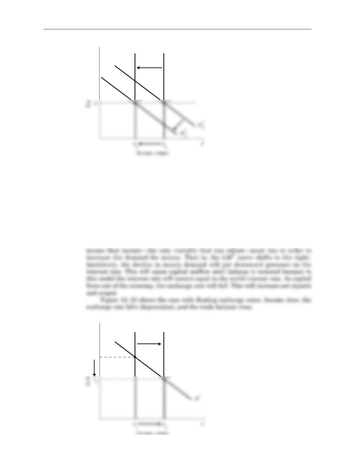
c. The introduction of ATM machines reduces the demand for money. We know that
equilibrium in the money market requires that the supply of real balances M/P
must equal demand:
M/P = L(r*, Y).
A fall in money demand means that for unchanged income and interest rates, the
right-hand side of this equation falls. Since Mand Pare both fixed, we know that
the left-hand side of this equation cannot adjust to restore equilibrium. We also
know that the interest rate is fixed at the level of the world interest rate. This
e
LM1
LM2
**
Figure 12–12
e
A
LM1LM2
e1
**
Figure 12–13
Chapter 12 Aggregate Demand in the Open Economy 127
Figure 12–14 shows the case of fixed exchange rates. The LM*schedule
shifts to the right; as before, this tends to push domestic interest rates down and
cause the currency to depreciate. However, the central bank buys dollars and sells
foreign currency in order to keep the exchange rate from falling. This reduces the
money supply and shifts the LM*schedule back to the left. The LM*curve contin-
ues to shift back until the original equilibrium is restored.
In the end, income, the exchange rate, and the trade balance are unchanged.
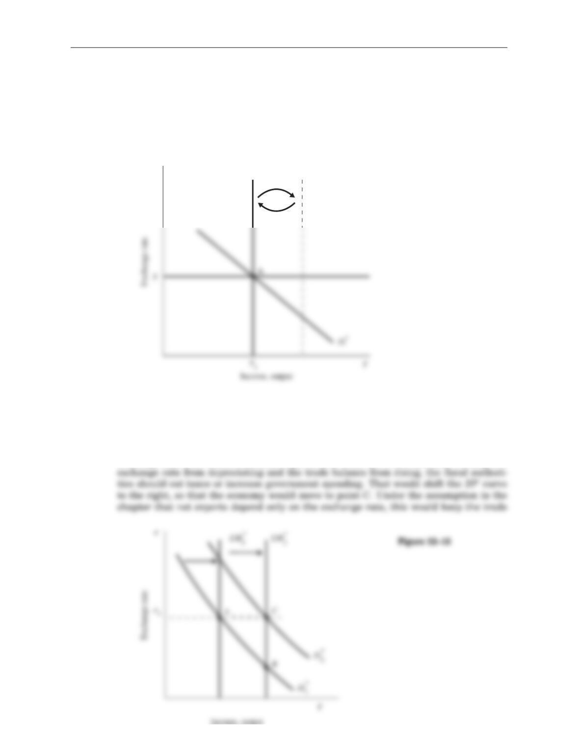
2. The economy is in recession, at point A in Figure 12–15. To increase income, the cen-
tral bank should increase the money supply, thereby shifting the
LM
* curve to the
right. If only that happened, the economy would move to point B, with a depreciated
exchange rate that would stimulate exports and raise the trade balance. To keep the
e
LM*
Figure 12–14
balance from changing. The increase in output and income would, instead, reflect an
increase in domestic demand. (Note that without the monetary expansion, a fiscal
expansion by itself would lead to a higher exchange rate—so the increase in domestic
demand would be offset by a reduction in the trade balance.
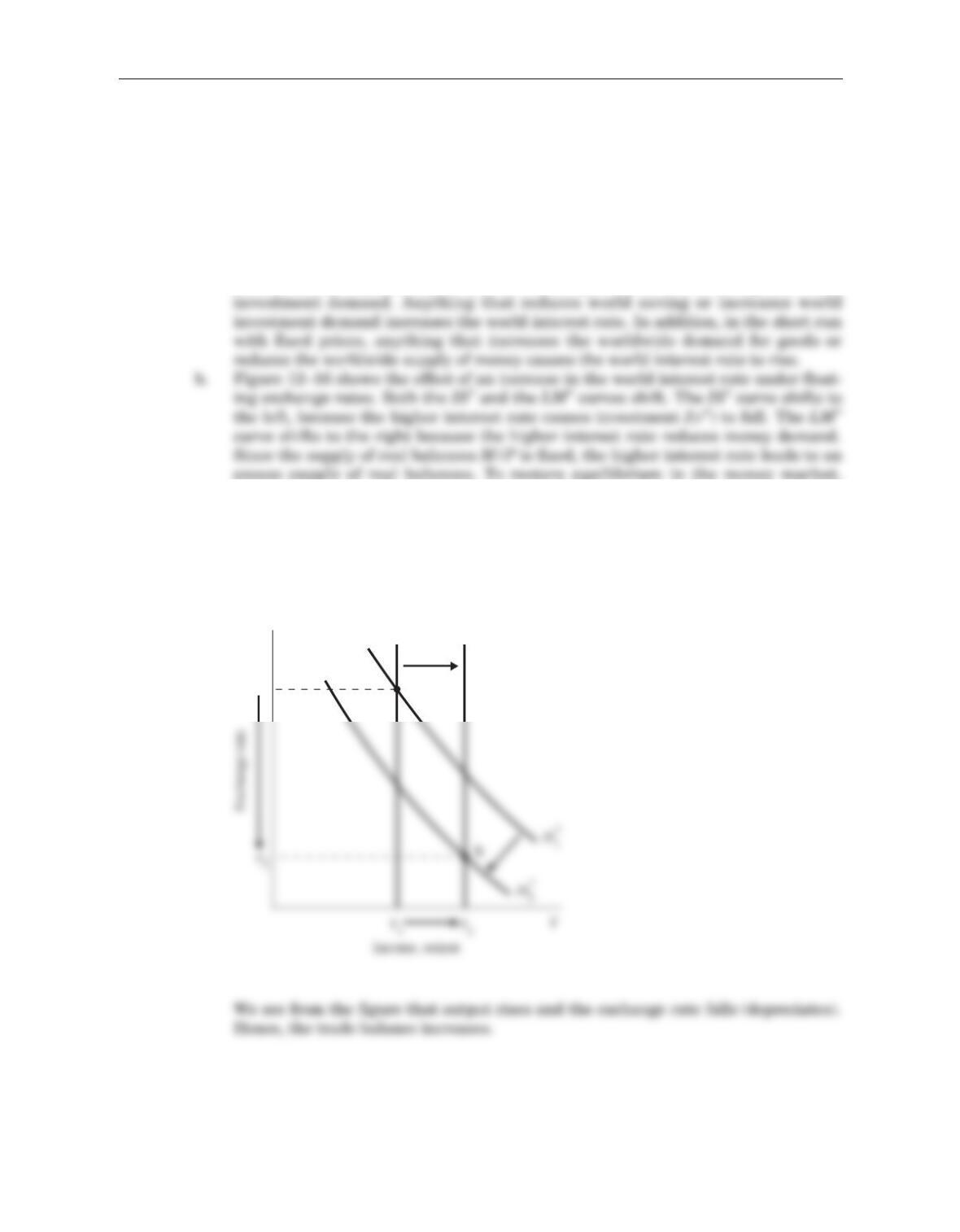
3. a. The Mundell–Fleming model takes the world interest rate r*as an exogenous
variable. However, there is no reason to expect the world interest rate to be con-
stant. In the closed-economy model of Chapter 3, the equilibrium of saving and
investment determines the real interest rate. In an open economy in the long run,
the world real interest rate is the rate that equilibrates world saving and world
income must rise; this increases the demand for money until there is no longer an
excess supply. Intuitively, when the world interest rate rises, capital outflow will
increase as the interest rate in the small country adjusts to the new higher level of
the world interest rate. The increase in capital outflow causes the exchange rate
to fall, causing net exports and hence output to increase, which increases money
demand.
128 Answers to Textbook Questions and Problems
e
A
LM
2
LM
1
e
1
* *
Figure 12–16
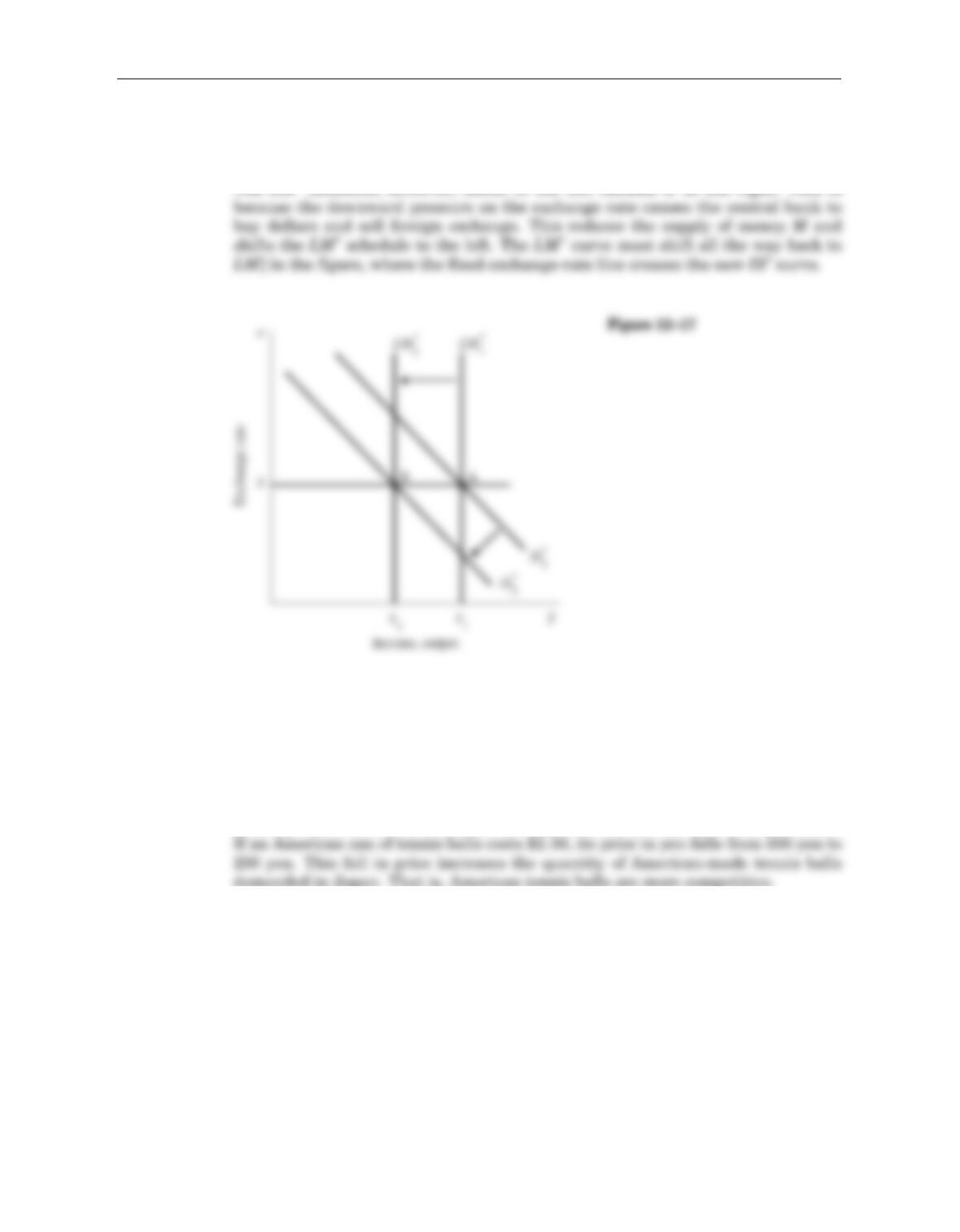
c. Figure 12–17 shows the effect of an increase in the world interest rate if exchange
rates are fixed. Both the IS*and LM*curves shift. As in part (b), the IS*curve
shifts to the left since the higher interest rate causes investment demand to fall.
In equilibrium, output falls while the exchange rate remains unchanged. Since the
exchange rate does not change, neither does the trade balance.
4. a. A depreciation of the currency makes American goods more competitive. This is
because a depreciation means that the same price in dollars translates into fewer
units of foreign currency. That is, in terms of foreign currency, American goods
become cheaper so that foreigners buy more of them. For example, suppose the
exchange rate between yen and dollars falls from 200 yen/dollar to 100 yen/dollar.
Chapter 12 Aggregate Demand in the Open Economy 129
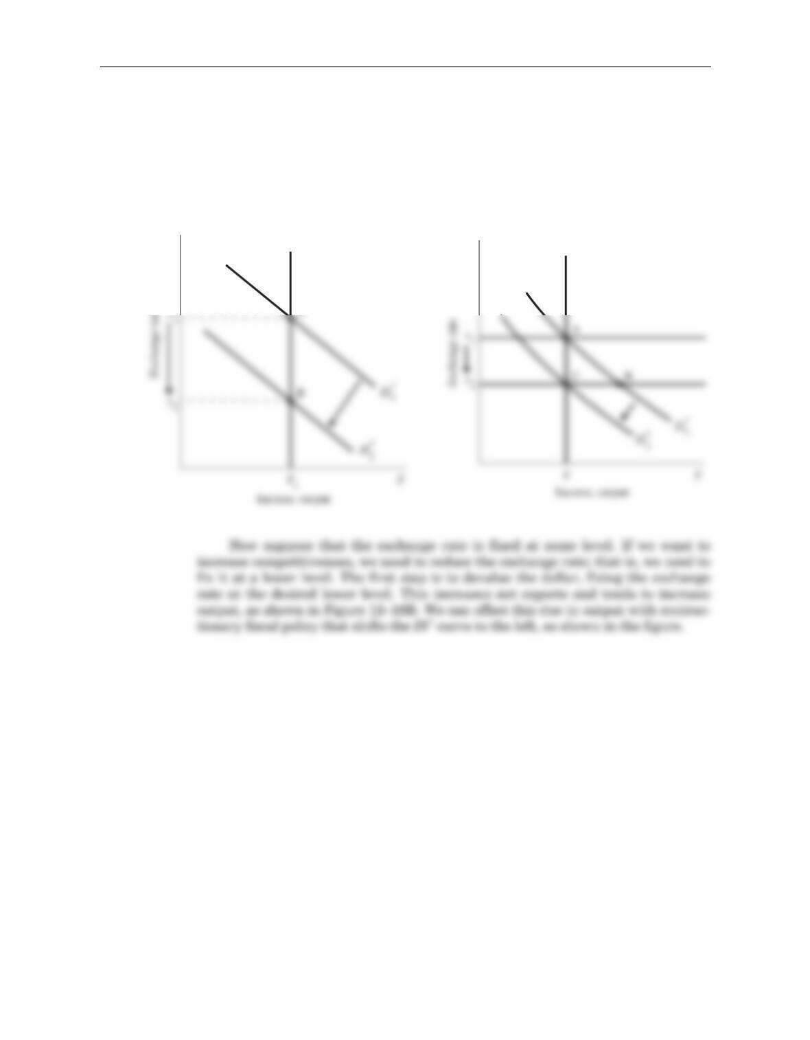
b. Consider first the case of floating exchange rates. We know that the position of the
LM*curve determines output. Hence, we know that we want to keep the money
supply fixed. As shown in Figure 12–18A, we want to use fiscal policy to shift the
IS*curve to the left to cause the exchange rate to fall (depreciate). We can do this
by reducing government spending or increasing taxes.
130 Answers to Textbook Questions and Problems
e
LM
*
e
LM*
Figure 12–18
A. Floating exchange rate B. Fixed exchange rates
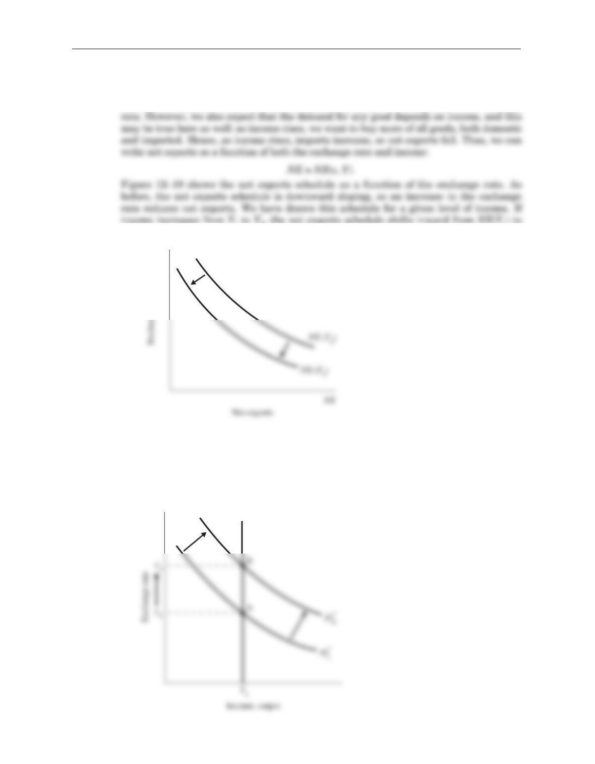
5. In the text, we assumed that net exports depend only on the exchange rate. This is analo-
gous to the usual story in microeconomics in which the demand for any good (in this case,
net exports) depends on the price of that good. The “price” of net exports is the exchange
NX(Y2).
a. Figure 12–20 shows the effect of a fiscal expansion under floating exchange rates.
The fiscal expansion (an increase in government expenditure or a cut in taxes)
shifts the IS*schedule to the right. But with floating exchange rates, if the LM*
curve does not change, neither does income. Since income does not change, the
net-exports schedule remains at its original level NX(Y1).
Chapter 12 Aggregate Demand in the Open Economy 131
e
Figure 12–19
e
LM*
Figure 12–20