Chapter 8: Risk and Rates of Return
Learning Objectives
189
Chapter 8
Risk and Rates of Return
Learning Objectives
After reading this chapter, students should be able to do the following:
◆ Explain the difference between stand-alone risk and risk in a portfolio context.
◆ Describe how risk aversion affects a stock’s required rate of return.
190
Lecture Suggestions
Chapter 8: Risk and Rates of Return
Lecture Suggestions
Risk analysis is an important topic, but it is difficult to teach at the introductory level. We just try to give
students an intuitive overview of how risk can be defined and measured, and leave a technical treatment
to advanced courses. Our primary goals are to be sure students understand (1) that investment risk is
the uncertainty about returns on an asset, (2) the concept of portfolio risk, and (3) the effects of risk on
required rates of return.
DAYS ON CHAPTER: 3 OF 56 DAYS (50-minute periods)
Answers to End-of-Chapter Questions
8-1 a. No, it is not riskless. The portfolio would be free of default risk and liquidity risk, but inflation
could erode the portfolio’s purchasing power. If the actual inflation rate is greater than that
expected, interest rates in general will rise to incorporate a larger inflation premium (IP)
and—as we saw in Chapter 6—the value of the portfolio would decline.
bonds.
8-2 a. The probability distribution for complete certainty is a vertical line.
8-3 a. The expected return on a life insurance policy is calculated just as for a common stock. Each
outcome is multiplied by its probability of occurrence, and then these products are summed.
For example, suppose a 1-year term policy pays $10,000 at death, and the probability of the
policyholder’s death in that year is 2%. Then, there is a 98% probability of zero return and a
2% probability of $10,000:
b. There is a perfect negative correlation between the returns on the life insurance policy and
the returns on the policyholder’s human capital. In fact, these events (death and future
lifetime earnings capacity) are mutually exclusive.
8-4 Yes, if the portfolio’s beta is equal to zero. In practice, however, it may be impossible to find
8-5 Security A is less risky if held in a diversified portfolio because of its negative correlation with
8-6 No. For a stock to have a negative beta, its returns would have to logically be expected to go up
in the future when other stocks’ returns were falling. Just because in one year the stock’s return
8-7 The risk premium on a high-beta stock would increase more than that on a low-beta stock.
RPj = Risk Premium for Stock j = (rM – rRF)bj.
8-8 According to the Security Market Line (SML) equation, an increase in beta will increase a
company’s expected return by an amount equal to the market risk premium times the change in
8-9 a. A decrease in risk aversion will decrease the return an investor will require on stocks. Thus,
prices on stocks will increase because the cost of equity will decline.
8-10 Investments with higher Sharpe ratios have performed better, because they have generated
higher excess returns per unit of risk. Therefore, Stock A has performed better than Stock B.
8-11 ABC’s realized return was 10%, which was higher than its required return of 9%. Therefore,
ABC’s stock plots above the SML and generates a positive alpha. If ABC’s realized return had
Solutions to End-of–Chapter Problems
8-1
r
ˆ
= (0.1)(-30%) + (0.1)(–14%) + (0.3)(11%) + (0.3)(20%) + (0.2)(45%)
= 13.90%.
8-2 Investment Beta
$20,000 0.6
8-3 rRF = 5.5%; rM = 12%; b = 2; r = ?
8-4 rRF = 3.5%; RPM = 4%; rM = ?
8-5 a. r = 9%; rRF = 4.5%; RPM = 3%.
r = rRF + (rM – rRF)b
194
Answers and Solutions
Chapter 8: Risk and Rates of Return
8-6 a.
=
=
N
1i
iirPr
ˆ
.
B
r
ˆ
= 0.1(-35%) + 0.2(0%) + 0.4(20%) + 0.2(25%) + 0.1(45%)
b. =
=
−
N
1i
i
2
iP)r
ˆ
r(
.
2
A
σ
= (-10% – 12%)2(0.1) + (2% – 12%)2(0.2) + (12% – 12%)2(0.4)
+ (20% – 12%)2(0.2) + (38% – 12%)2(0.1) = 148.8.
c. Sharpe ratio for Stock A = (12% − 2.5%)/12.20% = 0.7787.
Sharpe ratio for Stock B = (14% − 2.5%)/20.35% = 0.5651.
8-7 Portfolio beta =
0,00082$4,
0,0006$4
(1.50) +
0,00082$4,
00,0005$
(–0.50) +
0,00082$4,
0,00026$1,
(1.25) +
0,00082$4,
00,0006$2,
(0.75)
bp = (0.0954)(1.5) + (0.1037)(-0.50) + (0.2614)(1.25) + (0.5394)(0.75)
Stock Investment Beta r = rRF + (rM – rRF)b Weight
A $ 460,000 1.50 10% 0.0954
B 500,000 (0.50) 2 0.1037
8-8 In equilibrium:
rL =
L
r
ˆ
= 10.5%.
rL = rRF + (rM – rRF)b
8-9 We know that bR = 2.0, bS = 0.45, rM = 10%, rRF = 5%.
7.75%
8-10 An index fund will have a beta of 1.0. If rM is 11.0% (given in the problem) and the risk-free rate is
4.5%, you can calculate the market risk premium (RPM) calculated as rM – rRF as follows:
r = rRF + (RPM)b
8-11 rRF = r* + IP = 1.0% + 3.6% = 4.6%.
8-12 a. ri = rRF + (rM – rRF)bi = 4% + (10% – 4%)1.4 = 12.4%.
b. 1. rRF increases to 5%:
2. rRF decreases to 3%:
c. 1. rM increases to 12%:
ri = rRF + (rM – rRF)bi = 4% + (12% – 4%)1.4 = 15.2%.
8-13 a. Using Stock A (or any stock):
9.55% = rRF + (rM – rRF)bX
c. rP = 5.5% + 4.5%(1.2)
d. Since the returns on the 3 stocks included in Portfolio P are not perfectly positively correlated,
Chapter 8: Risk and Rates of Return
Answers and Solutions
197
8-14 Old portfolio beta =
$150,000
$142,500
(b) +
$150,000
$7,500
(1.00)
1.25 = 0.95b + 0.05
i
b
2.
i
b
excluding the stock with the beta equal to 1.0 is 25.0 – 1.0 = 24, so the beta of the
8-15 bHRI = 1.6; bLRI = 0.8. No changes occur.
rRF = 6%. Decreases by 1.5% to 4.5%.
8-16 Step 1: Determine the market risk premium from the CAPM:
0.11475 = 0.04 + (rM – rRF)1.15
(rM – rRF) = 0.065 = 6.5%.
198
Answers and Solutions
Chapter 8: Risk and Rates of Return
8-17 After additional investments are made, for the entire fund to have an expected return of 15%,
the portfolio must have a beta of 1.50 as shown below:
15% = 4.5% + (7%)b
b = 1.50.
Since the fund’s beta is a weighted average of the betas of all the individual investments, we can
calculate the required beta on the additional investment as follows:
1.50 =
000,000,25$
)7.1)(000,000,20($
+
000,000,25$
X000,000,5$
8-18 a. ($1 million)(0.5) + ($0)(0.5) = $0.5 million.
b. You would probably take the sure $0.5 million.
X
Y
r
ˆ
= 12.5%; bY = 1.2; Y = 25%.
rRF = 6%; RPM = 5%.
Chapter 8: Risk and Rates of Return
Answers and Solutions
199
X
ˆ
e. bp = ($7,500/$10,000)0.9 + ($2,500/$10,000)1.2
= 0.6750 + 0.30
= 0.9750.
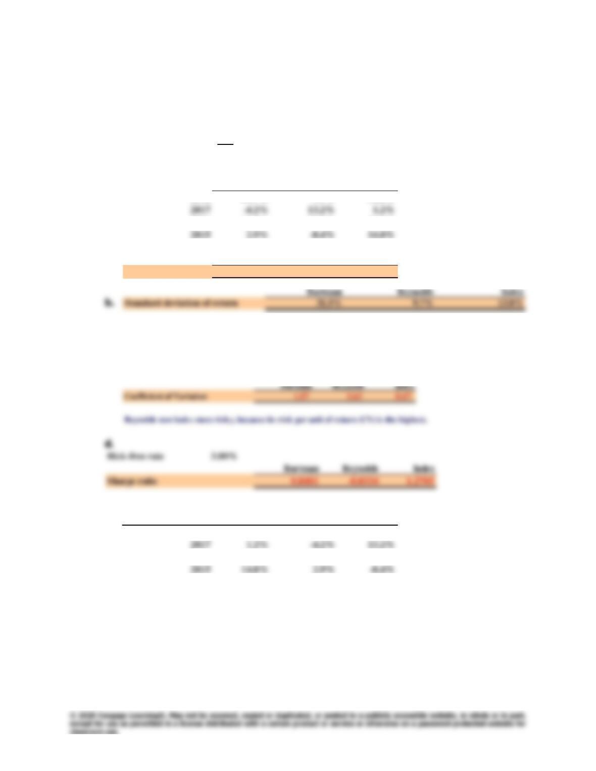
8-20 The answers to a, b, c, and d are given below:
rA rB Portfolio
2014 (18.00%) (14.50%) (16.25%)
2016 15.00 30.50 22.75
2017 (0.50) (7.60) (4.05)
Mean 11.30 11.30 11.30
e. A risk-averse investor would choose the portfolio over either Stock A or Stock B alone, since the
portfolio offers the same expected return but with less risk. This result occurs because returns
8-21 a.
M
r
ˆ
= 0.1(–28%) + 0.2(0%) + 0.4(12%) + 0.2(30%) + 0.1(50%) = 13%.
200
Answers and Solutions
Chapter 8: Risk and Rates of Return
b. First, determine the fund’s beta, bF. The weights are the percentage of funds invested in each
stock:
A = $160/$500 = 0.32.
c. rN = Required rate of return on new stock = 6% + (7%)1.5 = 16.5%.
An expected return of 15% on the new stock is below the 16.5% required rate of return on an
Chapter 8: Risk and Rates of Return
Comprehensive/Spreadsheet Problem
201
Comprehensive/Spreadsheet Problem
Note to Instructors:
The solution to this problem is not provided to students at the back of their text. Instructors
can access the
Excel
file on the textbook’s website.
8-22 a.
Bartman Reynolds Index
2018 24.7% –1.1% 32.8%
2016 62.8% –10.0% 34.9%
2014 61.0% 11.7% 19.0%
Avg Returns 29.5% 2.7% 20.6%
On a stand-alone basis, it would appear that Bartman is the most risky, Reynolds the least
risky.
c.
e.
Year Index Bartman Reynolds
2018 32.8% 24.7% –1.1%
2016 34.9% 62.8% –10.0%
2014 19.0% 61.0% 11.7%
Divide the standard deviation by the average return:
202
Comprehensive/Spreadsheet Problem
Chapter 8: Risk and Rates of Return
–20%
0%
10%
20%
70%
0.0% 10.0% 20.0% 30.0% 40.0%
Stocks’
Returns
Index Returns
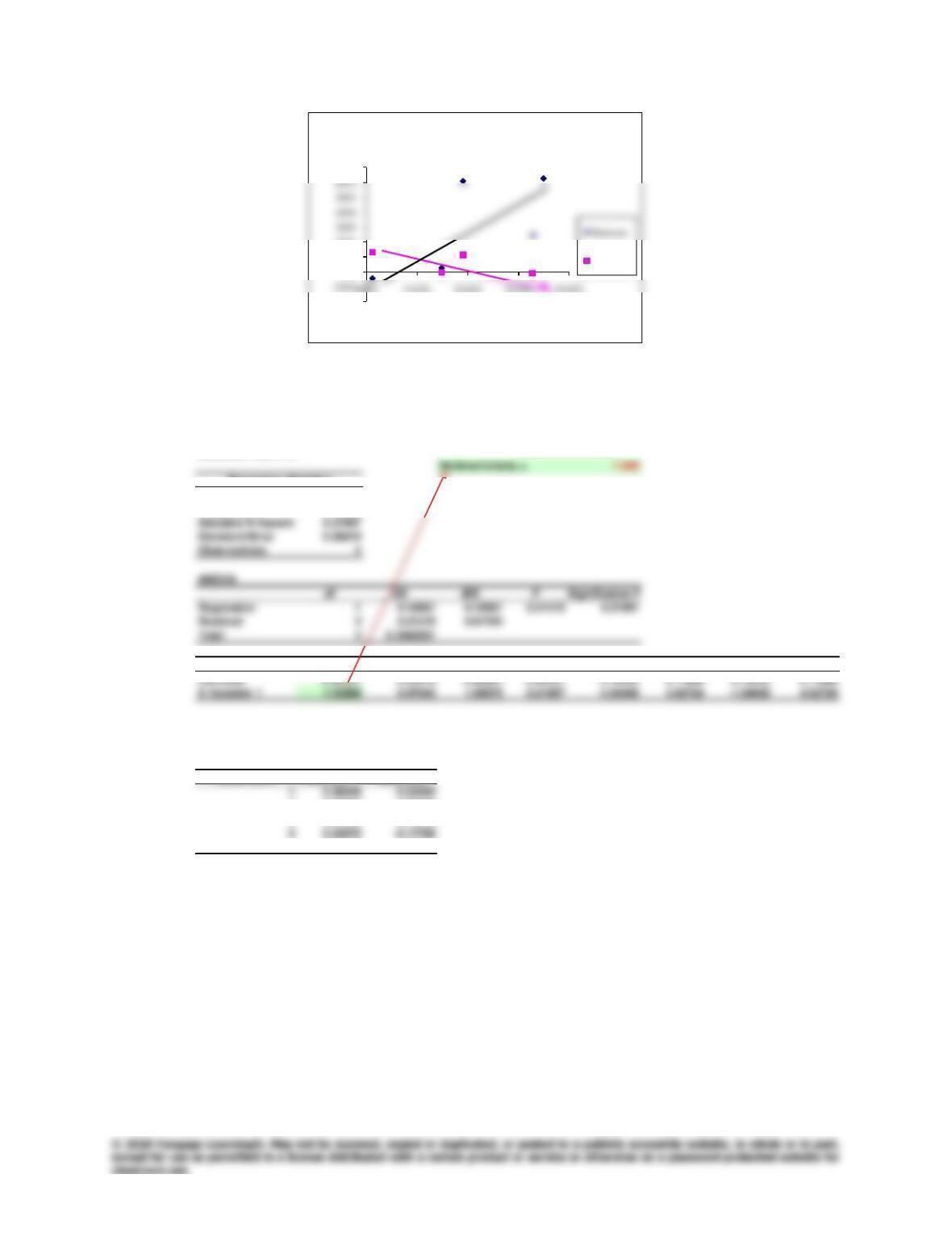
Stock Returns Vs. Index
Reynolds
It is clear that Bartman moves with the market and Reynolds moves counter to the market.
So, Bartman has a positive beta and Reynolds a negative one.
f. Bartman’s calculations:
SUMMARY OUTPUT
Regression Statistics
Multiple R 0.67528
R Square 0.45600
Coefficients
Standard Error
t Stat P-value Lower 95% Upper 95%
Lower 95.0%
Upper 95.0%
RESIDUAL OUTPUT
Observation Predicted Y Residuals
2 -0.00303 –0.03879
3 0.51542 0.11249
5 0.27133 0.33891
Chapter 8: Risk and Rates of Return
Comprehensive/Spreadsheet Problem
203
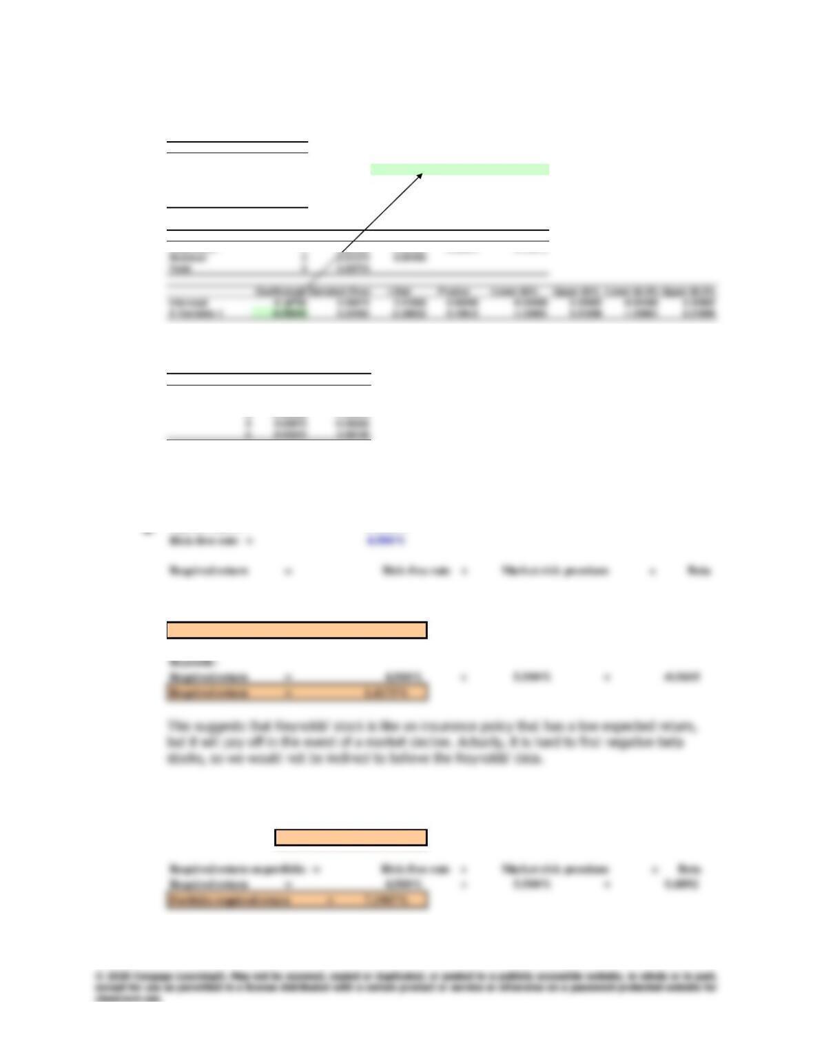
Reynolds’ calculations:
Note that these betas are consistent with the scatter diagrams we constructed earlier.
Reynolds’ beta suggests that it is less risky than average in a CAPM sense, whereas Bartman is
more risky than average.
g.
h. The beta of a portfolio is simply a weighted average of the betas of the stocks in the portfolio,
so this portfolio’s beta would be:
SUMMARY OUTPUT
Regression Statistics
Multiple R 0.79735
R Square 0.63576 Reynolds‘ beta = -0.560
Adjusted R Square 0.51435
Standard Error 0.06769
Observations 5
ANOVA
df SS MS F Significance F
Regression 1 0.02399 0.02399 5.23641 0.10612
RESIDUAL OUTPUT
Observation Predicted Y Residuals
1 -0.04165 0.03113
2 0.13514 -0.00283
3 -0.05368 -0.04676
Market return = 10.000%
Bartman:
Required return = 4.500% + 5.500% ×1.5389
Required return = 12.9639%
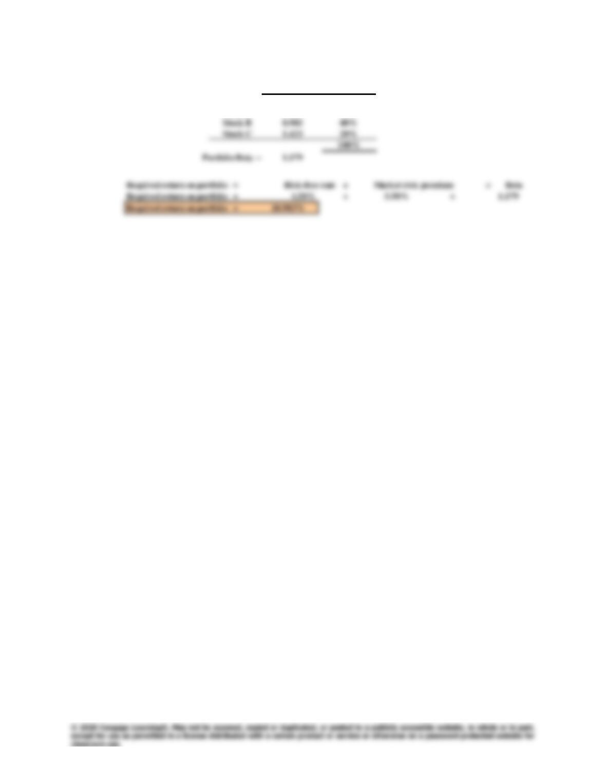
Portfolio beta =
0.4892
204
Comprehensive/Spreadsheet Problem
Chapter 8: Risk and Rates of Return
i.
Beta
Portfolio
Weight
Bartman 1.539 25%
Stock A 0.769 15%
Chapter 8: Risk and Rates of Return
Integrated Case
205
Integrated Case
8-23
Merrill Finch Inc.
Risk and Return
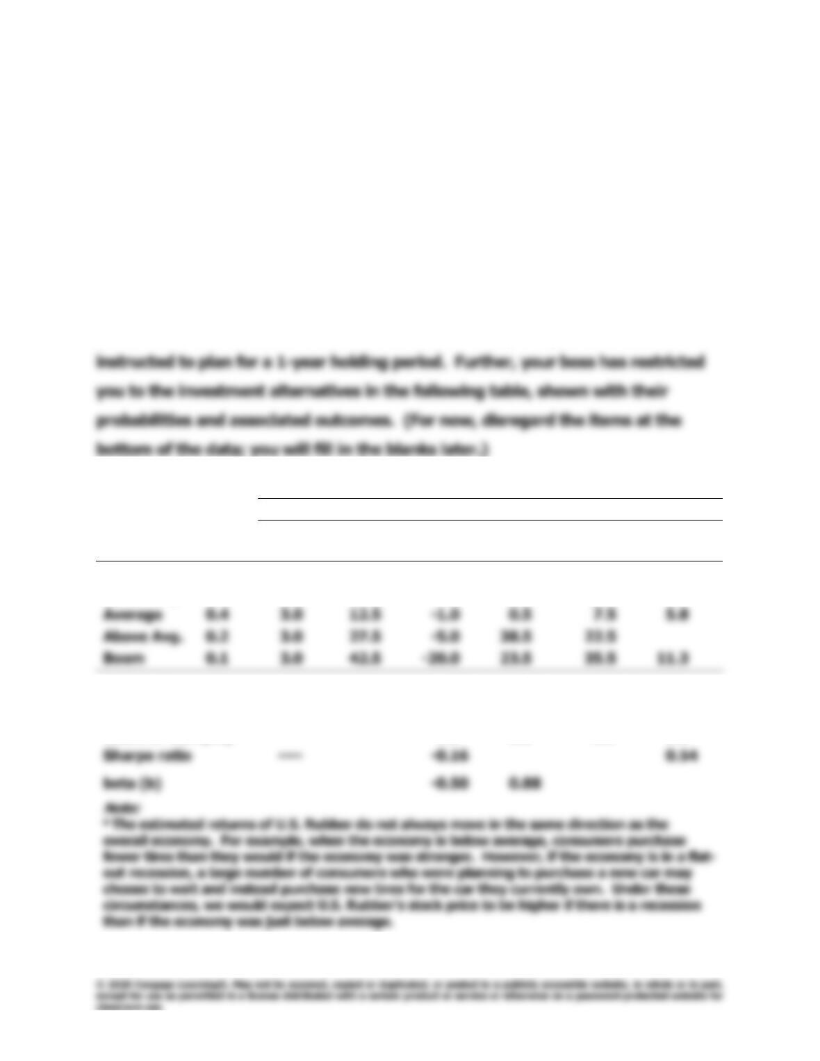
Assume that you recently graduated with a major in finance. You just landed a
job as a financial planner with Merrill Finch Inc., a large financial services
corporation. Your first assignment is to invest $100,000 for a client. Because the
funds are to be invested in a business at the end of 1 year, you have been
Returns on Alternative Investments
Estimated Rate of Return
State of the
Economy
Prob.
T-Bills
High
Tech
Collec-
tions
U.S.
Rubber
Market
Portfolio
2-Stock
Portfolio
Recession
0.1
3.0%
-29.5%
24.5%
3.5%a
-19.5%
-2.5%
Below Avg.
0.2
3.0
-9.5
10.5
-16.5
-5.5
Average
0.4
3.0
12.5
-1.0
0.5
7.5
5.8
Above Avg.
0.2
3.0
27.5
-5.0
38.5
22.5
Boom
0.1
3.0
42.5
-20.0
23.5
35.5
11.3
r-hat (
r
ˆ
)
1.2%
7.3%
8.0%
Std. dev. ()
0.0
11.2
18.8
15.2
4.6
Coeff. of Var. (CV)
9.8
2.6
1.9
0.8
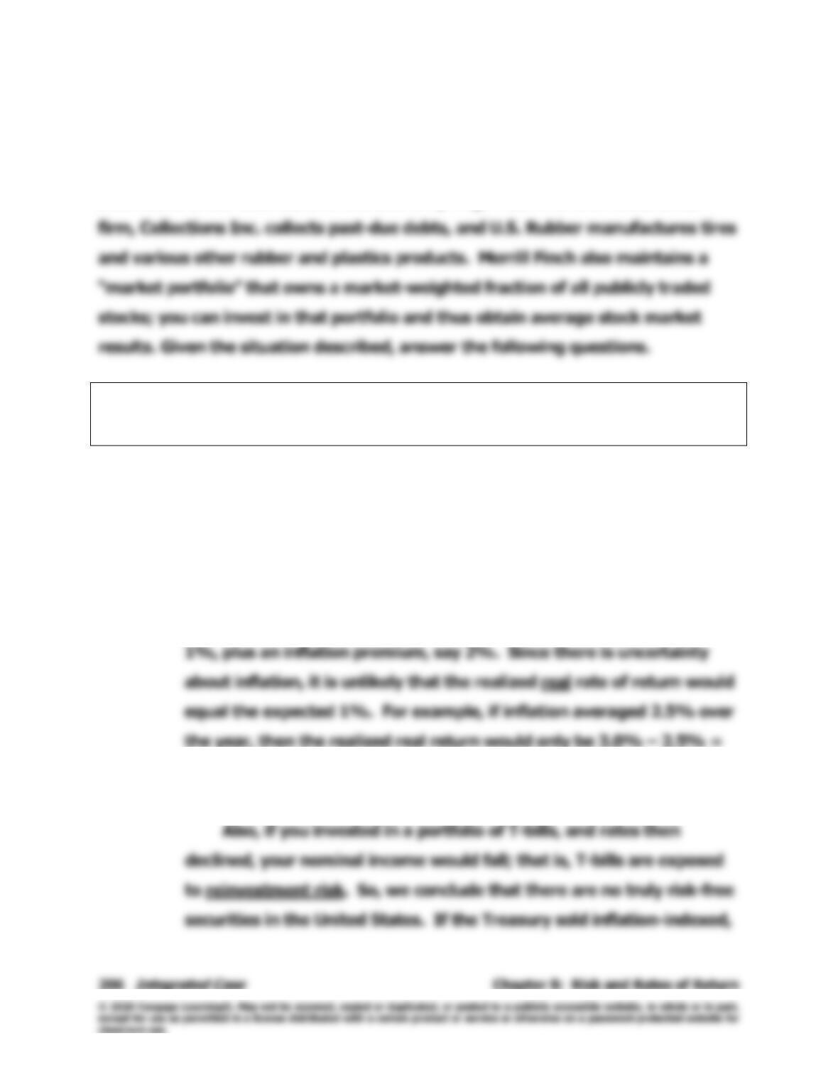
Merrill Finch’s economic forecasting staff has developed probability
estimates for the state of the economy, and its security analysts developed a
sophisticated computer program to estimate the rate of return on each
alternative under each state of the economy. High Tech Inc. is an electronics
A. (1) Why is the T-bill’s return independent of the state of the economy?
Do T-bills promise a completely risk-free return? Explain.
Answer: [Show S8-1 through S8-7 here.] The 3.0% T–bill return does not
depend on the state of the economy because the Treasury must (and
will) redeem the bills at par regardless of the state of the economy.
The T-bills are risk free in the default risk sense because the
3.0% return will be realized in all possible economic states. However,
remember that this return is composed of the real risk-free rate, say
0.5%, not the expected 1%. Thus, in terms of purchasing power,
T–bills are not riskless.