Chapter 12
Consumption, Real GDP, and the Multiplier
◼ Overview
The main objective of this chapter is to indicate how macroeconomic equilibrium is attained in a Keynesian
framework. The income–expenditure model is developed. In the process, the concepts of consumption,
saving, investment, and net exports are developed and used to derive macroeconomic equilibrium. Another
important objective is to derive and explain the significance of the multiplier both in the fixed price model
and in the AS–AD model. Finally, the chapter shows how C + I + G + X is related to aggregate demand.
◼ Learning Objectives
After studying this chapter, students should be able to:
• 12.1 Explain the key determinants of consumption and saving in the Keynesian model
◼ Outline
I. Determinants of Planned Consumption and Planned Saving: We assume that the short-run
aggregate supply curve is horizontal so that the equilibrium level of real GDP is demand determined.
A. Some Simplifying Assumptions in a Keynesian Model: (1) Businesses pay no indirect taxes,
1. Another Look at Definitions and Relationships: Consumption is the act of using income
for the purchase of consumption goods. Consumption goods are goods purchased by
households for immediate satisfaction. By definition, whatever is not consumed is saved.
a. Stocks and Flows: The Difference between Saving and Savings: It is important to
2. Investment Spending: A flow concept that includes fixed investment, which is defined as
B. How Income Flows Can Influence Consumption and Saving
2. The Permanent Income Hypothesis: A theory in which consumption decisions depend on
3. The Keynesian Theory of Consumption: Keynes argues that consumption decisions
4. Graphing the Numbers (See Figure 12-1.)
a. Consumption and Saving Functions: The consumption and saving functions show
5. Dissaving and Autonomous Consumption: Dissaving is negative saving. It is a situation
where spending exceeds income.
6. Average Propensity to Consume and to Save: Average propensity to consume (APC) is
7. Marginal Propensity to Consume and to Save: Marginal propensity to consume (MPC)
is change in real consumption divided by change in disposable income. Marginal
propensity to save (MPS) is change in real saving divided by change in real disposable
8. Some Relationships
9. Causes of Shifts in the Consumption Function: Whenever there is a change in non-
172 Miller • Economics Today, Nineteenth Edition
II. Determinants of Investment: Investment is defined as expenditures on new plant, capital
equipment, and changes in business inventories. Real gross private domestic investment in the
United States has been volatile compared to real consumption because investment decisions of
business people are based on highly variable, subjective expectations of the economic future.
A. The Planned Investment Function: At all times, businesses perceive an array of investment
B. What Causes the Investment Function to Shift? If non-interest rate determinants of
III. Determining Equilibrium Real GDP: Net taxes average about 18 percent of real GDP. Assuming
that real disposable income differs from real GDP by the same absolute amount every year, real
GDP can be substituted for real disposable income in the consumption function. (See Figure 12-3.)
A. Consumption as a Function of Real GDP: The model of consumption is simplified by
B. The 45-Degree Reference Line: The line along which planned consumption expenditures are
equal to real GDP, or C = Y.
C. Adding the Investment Function: In the simplified Keynesian model, real investment per year
is assumed to be autonomous with respect to real GDP. (See Figure 12-4.)
2. Combining Planned Investment and Consumption: The consumption plus investment
D. Saving and Investment: Planned versus Actual: Equilibrium occurs at the intersection of the
planned saving and planned investment schedules. There is no tendency for businesses to alter
1. Unplanned Changes in Business Inventories
a. A Mismatch between Actual and Anticipated Purchases: If consumers buy less
b. How Businesses Adjust: Businesses respond to a rise in unplanned inventories by
Chapter 12 Consumption, Real GDP, and the Multiplier 173
IV. Keynesian Equilibrium with Government and the Foreign Sector Added (See Table 12-2.)
B. The Foreign Sector: The level of exports depends on international economic conditions in the
V. The Multiplier, Total Expenditures, and Aggregate Demand: The multiplier is the number
by which a permanent change in autonomous spending, such as autonomous investment or
A. The Multiplier Effect: The autonomous spending multiplier is directly related to the MPC and
inversely related to the MPS. The change in the equilibrium level of real national income due to
a change in autonomous spending is the multiplier times the change in autonomous spending.
(See Table 12-3.)
2. The Multiplier Process: As household income increases, induced consumption spending
B. The Multiplier Formula: Multiplier = 1/(1 − MPC) = 1/MPS. The multiplier effect due to
permanent change in autonomous spending is given by the formula:
1. Determining the Multiplier with Either MPC or MPS: Because MPC + MPS = 1, we
2. How the Values of MPC and MPS Affect the Multiplier: The smaller the marginal
D. How a Change in Real Autonomous Spending Affects Real GDP When the Price Level
(See Figure 12-7.)
2. Accounting for a Price Level Change: The price level does not stay fixed because SRAS
174 Miller • Economics Today, Nineteenth Edition
E. The Relationship between Aggregate Demand and the C + I + G + X Curve: The C + I +
◼ Points to Emphasize
Macroeconomic Equilibrium
Equilibrium should be presented as a behavioral concept. It occurs when plans are realized. If the 45-degree
reference line is viewed as a planned-expenditures-equals-real-GDP line, then equilibrium occurs when
Equilibrium and Unemployment
One of Keynes’s main contributions to macroeconomic analysis was his demonstration of the simultaneous
existence of unemployment and equilibrium. Keynesian equilibrium is at the point of intersection of the
planned saving and investment curves. The question is whether there is full employment at this equilibrium
The Multiplier
In describing the multiplier effect, stress the importance of shifts in the planned expenditure, or C + I +
Chapter 12 Consumption, Real GDP, and the Multiplier 175
in the curve will cause the equilibrium level of income to fall by more than $1.00. The multiplier can
Consumption has increased by 75 cents, and Y has increased by 75 cents because those people who
produced and sold the 75 cents worth of goods (bought by those people who produced and sold the
$1.00 machine) have now received an increase in income.
◼ For Those Who Wish to Stress Theory
Mathematical Equilibrium
Having already presented the graphical exposition of equilibrium determination, a simple algebraic
approach to equilibrium can be shown. Assume a Keynesian consumption function:
176 Miller • Economics Today, Nineteenth Edition
Substituting from Equations (1) and (2) into Equation (3) yields
Q = Y = (a + by) + I = E (4)
Multiplier Size
The size of the multiplier is considerably smaller than the reciprocal of the MPS. Leaving aside leakages
to the foreign and government sectors, there still remains the restraining effect of price level changes.
The Keynesian versus the Classical Model
The leakage-injection approach allows comparison of the Keynesian and the classical models. In the
classical model, equilibrium exists at the point where saving and investment schedules intersect. The interest
Chapter 12 Consumption, Real GDP, and the Multiplier 177
If starting from full-employment equilibrium, the entire saving function shifts downward; the community
is saving more at every rate of interest. There is a surplus of saving, and interest rates fall to a lower
◼ Further Questions for Class Discussion
1. In 2008 and 2009, households that were able were encouraged by financial advisors to increase
their savings to make it possible for them to be prepared for possibly very uncertain financial
future. The saving rate increased from 4.9 percent to 6.1 percent. Is it possible that this advice
and the subsequent following of it by millions of Americans had any relationship to the severity
2. Why is the size of the multiplier important? The size of the multiplier determines by how much the
3. Why is the 45-degree line equal to the value of real GDP and the sum of planned real consumption,
investment, government expenditure, and net exports in equilibrium? Actual and realized real GDP
4. In late 2008 through the first two quarters of 2009, the rate of saving out of disposable income
increased. In the simple Keynesian model (no government of foreign transaction), what would this
5. Throughout the early 2000s, imports increased faster than exports. Explain the effect of this trend
on the C + I + G + X curve and on the aggregate demand (AD) curve. If imports increased faster
◼ Answers to Questions for Critical Analysis
What the Media Actually Report about When Describing Variations in the
“Saving Rate” (p. 260)
When the average propensity to save declines as real disposable income increases, what must
happen to the average propensity to consume? Explain your reasoning.
Diminished Rightward Shifts in Germany’s Investment Function (p. 264)
In principle, what might be possible causes of the observed diminishment of the rightward shifts of
Germany’s investment function over time? (Hint: Recall that changes in productive technology of
business taxes affect levels of planned investment spending)
Habit Formation in Consumption Spending and the Multiplier Effect (p. 270)
In light of the above discussion, how is a greater degree of habit persistence in consumption likely
to affect the marginal propensity to save? Explain your reasoning.
◼ You Are There
Inferring Low Real GDP Growth from “Restrained” Consumption Spending (p. 273)
1. According to Keynesian theory, what should have determined the actual amount of the
response of real consumption expenditures to the small increase in real GDP?
2. What does the theory of consumption spending predict should have happened to real saving
during the particular three-month period that Price was considering? Explain briefly.
◼ Issues and Applications
An Investment Spending Slowdown Holds Down U.S. Real GDP (pp. 274–275)
1. How could toughened federal regulations of businesses during the current decade have
inhibited a rightward shift in the investment function?
2. How might recent increases in state and federal tax rates on incomes that businesses derive
from capital investment have contributed to the investment function’s failure to rebound?
◼ Research Project
Appendix C—The Keynesian Model and Multiplier
The multiplier effect of can be observed in the Keynesian model as successive rounds of additional
spending induced by an autonomous increase in planned expenditures. (See Figure C-1.)
◼ Answers to Problems
12-1. Classify each of the following as either a stock or a flow.
a. Myung Park earns $850 per week.
b. Time Warner purchases $100 million in new telecommunications equipment this month.
c. Sally Schmidt has $1,000 in a savings account at a credit union.
d. XYZ, Inc., produces 200 units of output per week.
e. Giorgio Giannelli owns three private jets.
f. Apple’s production declines by 750 digital devices per month.
g. Russia owes $25 billion to the International Monetary Fund.
180 Miller • Economics Today, Nineteenth Edition
12-2. Consider the table below when answering the following questions. For this hypothetical
economy, the marginal propensity to save is constant at all levels of real GDP, and
investment spending is autonomous. There is no government.
Real GDP
Consumption
Saving
Investment
$ 2,000
$2,200
$______
$400
4,000
4,000
______
______
6,000
______
______
______
8,000
______
______
______
10,000
______
______
______
12,000
______
______
______
a. Complete the table. What is the marginal propensity to save? What is the marginal
propensity to consume?
b. Draw a graph of the consumption function. Then add the investment function to obtain
C + I.
c. Under the graph of C + I, draw another graph showing the saving and investment
curves. Note that the C + I curve crosses the 45-degree reference line in the upper graph
at the same level of real GDP where the saving and investment curves cross in the lower
graph. (If not, redraw your graphs.) What is this level of real GDP?
d. What is the numerical value of the multiplier?
e. What is equilibrium real GDP without investment? What is the multiplier effect from
the inclusion of investment?
f. What is the average propensity to consume at equilibrium real GDP?
g. If autonomous investment declines from $400 to $200, what happens to equilibrium
real GDP?
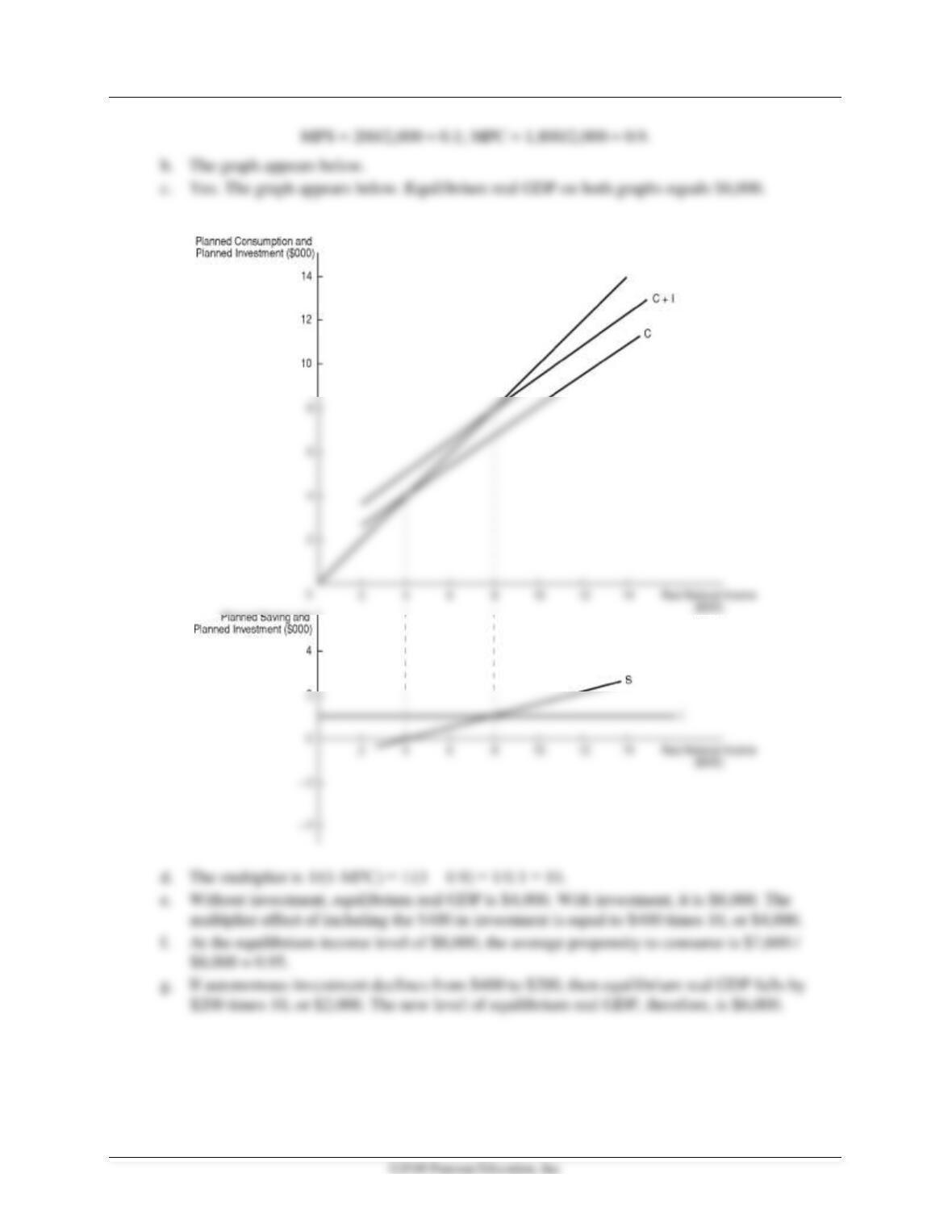
a. The completed table follows (all amounts in dollars):
Real GDP
Consumption
Saving
Investment
2,000
2,200
–200
400
4,000
4,000
400
6,000
5,800
400
8,000
7,600
400
Chapter 12 Consumption, Real GDP, and the Multiplier 181
12-3. Consider the table below when answering the following questions. For this economy, the
marginal propensity to consume is constant at all levels of real GDP, and investment
spending is autonomous. Equilibrium real GDP is equal to $8,000. There is no government.
182 Miller • Economics Today, Nineteenth Edition
Real GDP
Consumption
Saving
Investment
$ 2,000
$ 2,000
______
______
4,000
3,600
______
______
6,000
5,200
______
______
8,000
6,800
______
______
10,000
8,400
______
______
12,000
10,000
______
______
a. Complete the table. What is the marginal propensity to consume? What is the marginal
propensity to save?
b. Draw a graph of the consumption function. Then add the investment function to
obtain C + I.
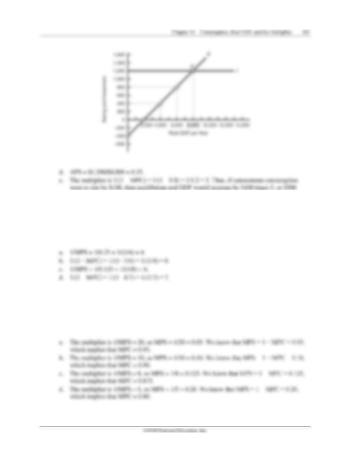
c. Under the graph of C + I, draw another graph showing the saving and investment
curves. Does the C + I curve cross the 45-degree reference line in the upper graph at the
same level of real GDP where the saving and investment curves cross in the lower graph,
at the equilibrium real GDP of $8,000? (If not, redraw your graphs.)
d. What is the average propensity to save at equilibrium real GDP?
e. If autonomous consumption were to rise by $100, what would happen to equilibrium
real GDP?
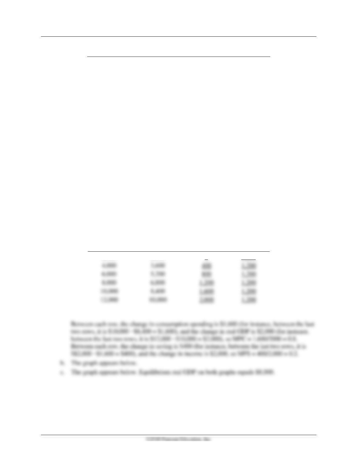
a. The completed table follows (all amounts in dollars):
Real GDP
Consumption
Saving
Investment
2,000
2,000
0
1,200
4,000
3,600
1,200
6,000
5,200
1,200
8,000
6,800
1,200
1,200
8,400
1,600
1,200
2,000
1,200
12-4. Calculate the multiplier for the following cases.
a. MPS = 0.25
b. MPC = 5/6
c. MPS = 0.125
d. MPC= 6/7
12-5. Given each of the following values for the multiplier, calculate both the MPC and the MPS.
a. 20
b. 10
c. 8
d. 5
12-6. The marginal propensity to consume is equal to 0.80. An increase in household wealth causes
autonomous consumption to rise by $10 billion. By how much will equilibrium real GDP
increase at the current price level, other things being equal?
12-7. Assume that the multiplier in a country is equal to 4 and that autonomous real consumption
spending is $1 trillion. If current real GDP is $18 trillion, what is the current value of real
consumption spending?
12-8. The multiplier in a country is equal to 5, and households pay no taxes. At the current
equilibrium real GDP of $14 trillion, total real consumption spending by households is
$12 trillion. What is real autonomous consumption in this country?
12-9. At an initial point on the aggregate demand curve, the price level is 125, and real GDP is
$18 trillion. When the price level falls to a value of 120, total autonomous expenditures
increase by $250 billion. The marginal propensity to consume is 0.75. What is the level
of real GDP at the new point on the aggregate demand curve?
12-10. At an initial point on the aggregate demand curve, the price level is 100, and real GDP is $18
trillion. After the price level rises to 110, however, there is an upward movement along the
aggregate demand curve, and real GDP declines to $14 trillion. If total planned spending
declined by $200 billion in response to the increase in the price level, what is the marginal
propensity to consume in this economy?
12-11. In an economy in which the multiplier has a value of 3, the price level has decreased from
115 to 110. As a consequence, there has been a movement along the aggregate demand curve
from $18 trillion in real GDP to $18.9 trillion in real GDP.
a. What is the marginal propensity to save?
b. What was the amount of the change in planned expenditures generated by the decline in
the price level?
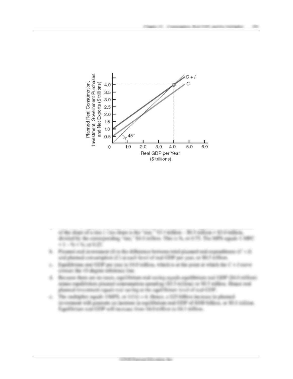
12-12. Consider the diagram below, which applies to a nation with no government spending, taxes,
and net exports. Use the information in the diagram to answer the following questions, and
explain your answers.
a. What is the marginal propensity to save?
b. What is the present level of planned investment spending for the present period?
c. What is the equilibrium level of real GDP for the present period?
d. What is the equilibrium level of saving for the present period?
e. If planned investment spending for the present period increases by $25 billion, what will
be the resulting change in equilibrium real GDP? What will be the new equilibrium level
of real GDP if other things, including the price level, remain unchanged?
a. The MPC is equal to the slope of the consumption function. (See Appendix A for discussion
12-13. Consider movements from points F to K in both panels of Figure 12-1. Use the resulting
changes in planned real consumption and saving corresponding to the change in real
disposable income to calculate the marginal propensity to consume and to save.
12-14. Take a look at Figure 12-5. If current real GDP for this nation’s economy is $13 trillion per
year, what are the values of planned real investment and actual real investment? What is the
amount of the unplanned inventory change, and why does this fact imply that real GDP must
change? To what new level will real GDP adjust?
12-15. Consider Table 12-2. What is the average propensity to consume at the equilibrium level of
real GDP? What is the average propensity to save?
12-16. Take a look at Table 12-2 and consider the changes in planned real consumption and saving
associated with an increase in real GDP from $14.0 trillion to $15.0 trillion to calculate the
marginal propensity to consume.
12-17. Consider the current equilibrium real GDP level of $18.0 trillion displayed in Table 12-2.
Based on your answer to Problem 4, if real government spending were to decrease by $1.0
trillion, what would be the resulting change in real GDP? What would be the new
equilibrium level of real GDP? Verify that at the new level of government spending, this new
equilibrium real GDP equals C + I + G + X.
12-18. Consider Figure 12-7, which applies to an economy in which the marginal propensity to
consume is 0.8. Why does a $0.1 trillion increase in planned real investment spending cause
the aggregate demand curve to shift rightward by exactly $0.5 trillion at the initial
equilibrium price level of 110?
12-19. Following the rightward shift in the aggregate demand curve generated by the $0.1 trillion
rise in real planned investment spending in Problem 12-18, why does the actual equilibrium
level of real GDP increase by only $0.3 trillion instead of $0.5 trillion?
◼ Selected References
Ackley, Gardner, Macroeconomics: Theory and Policy, New York: Macmillan, 1978.
Ando, A. and F. Modigliani, “Velocity and the Investment Multiplier,” American Economic Review,
Vol. LV, No. 4, September 1965, pp. 693–728, 786–790.