Basic Econometrics, Gujarati and Porter
144
CHAPTER 12:
AUTOCORRELATION: WHAT HAPPENS IF THE ERROR TERMS
ARE CORRELATED?
12.1 (a) False. The estimators are unbiased but they are not efficient.
12.2
For n = 50 and k‘ = 4, and α = 5%, the critical d values are:
d
L
= 1.38 4 – d
L
= 2.62
d
U
= 1.72 4 – d
U
= 2.28
12.3
(a) There is serial correlation in Model A, but not in Model B.
12.4
(a) Compute the Von Neumann (V-N) ratio, its mean, and its
variance.
Basic Econometrics, Gujarati and Porter
(e)
Given n = 100, the mean and variance of the V-N ratio can be
12.6
Dividing the numerator and denominator by n
2
, we obtain:
2
d k
12.7
(a) The main advantage is simplicity. It can also handle problems
12.8
(a) Using Minitab software, it took about 4 iterations to find a stable
(b) The new regression results are:
Basic Econometrics, Gujarati and Porter
146
The results when leaving correcting for the first observation (instead of
leaving it out) are as follows:
12.9
Using the ρ estimated from Eq. (3) of the C-O procedure, it can be
12.10
(a) The regression results are as follows:
Variable Coefficient Std. Error t-Statistic Prob.
R-squared 0.996340 Mean dependent var 91.11111
From the coefficient of Y
t-1
, we see that
ˆ
ρ
= 0.8795, which is not much different
147
12.11
(a) The figure shows that there is probably specification bias due to
12.12
(a) There are many reasons for an outlier. It may be an observation
12.13
See answer to Exercise 12.3
12.14
1
2 2
1 1
var( ) [( )( )] (1 )
t t t
t t t t t
E u u u u
ε ρ ρ ρ σ
−
− −
= − − = +
12.15
Since the model contains the lagged dependent variable as a
12.16
Given the AR(1) scheme,
12.17
Transform the model as follows:
1 1 2 2 1 1 2 2 1 1 2 2
( ) (1 ) ( )
t t t t t t t
Y Y Y X X X
ρ ρ β ρ ρ β ρ ρ ε
− − − −
− − = − − + − − +
2 2 2 2
1 1 1 1 1 1
( ) [(1 ) ] ( )( )[(1 ) ]
t t t t t t
x x x y x x y y x
ρ ρ ρ ρ ρ
− − −
∑
− − −
∑
− − −
12.19
Start with (12.9.6), which in deviation form can be written as:
* * *
12.20
This sequence has 22 positive signs and 11 negative signs. The
number of runs is 14. Using the normal approximation given in the
12.21
The formula would be:
2
n
149
12.22
As noted in the text, if there is an intercept term in the first difference
regression, it means that there was a linear trend term in the original
12.23
Since, ˆ
1 1
d
ρ
≈ − ≈
when d is very small. In that case the
12.24
If r = 0, Eq. (12.4.1) reduces to:
2
2
2
2
( )
2
1
n
σσ
ρ
−−
12.25 (a) As you can see from the computer output, only the residual at
Empirical Exercises
12.26 (a) The estimated regression is as follows:
Basic Econometrics, Gujarati and Porter
150
(c)As shown in the regression output given in (a) above, the d
(d) For the runs test, n = 30, n
1
= 17 , n
2
= 13, and R =9. From the
12.27 The regression results are:
ˆ
246.240 15.182
t t
Y X
= +
(b)
Yes. For n = 15, k‘ = 1 and α = 0.05, d
L
= 1.077. Since
(c)
(i): The Theil-Nagar statistic (see Exercise 12.6) for n = 15 and
151
* *
ˆ
32.052 19.404
Y X
= +
(e) Although the d value of 1.923 may suggest that there is no
autocorrelation, it is not clear if the Durbin-Watson d is appropriate
12.28
(a) The regression results for the C-O two stage procedure are:
* * * *
*
ˆ
1.214 0.398ln 0.336 ln 0.055ln 0.456 ln
t
i t t t
Y I L H A
= − + + − +
(b) The estimated
ρ
value from the C-O two-step procedure is 0.524,
12.29
The results of the linear total cost regression are:
ˆ
166.4667 19.933
i t
Y X
= +
12.30
The regression results in the level form are already given in Problem
7.21.That regression shows that the d value is 0.2187, which is quite
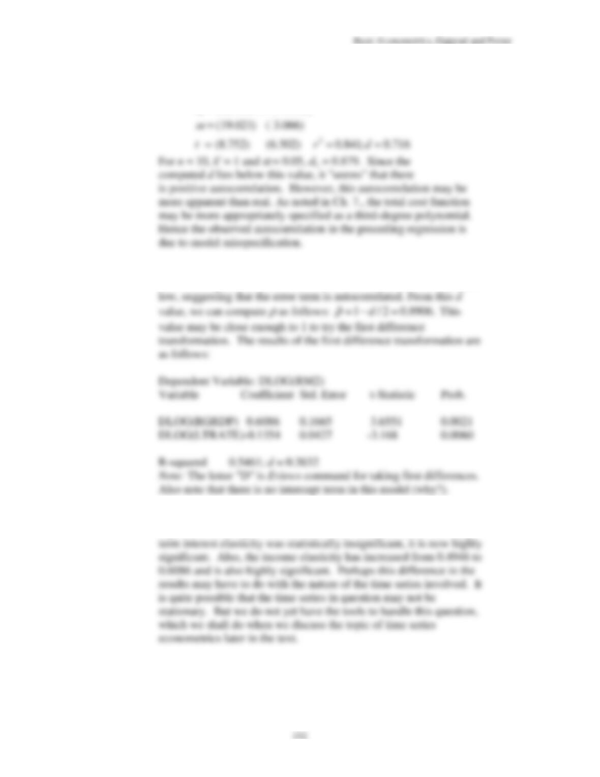
The results of this regression are interesting compared to the original
regression results given in Problem 7.21. Whereas before the long-
12.31
Since the X values are already arranged in the ascending order, the
computed d value and the d value computed by the procedure
Basic Econometrics, Gujarati and Porter
153
12.32
The regression results are already given in Problem 11.22. For this
regression the estimated d value is 2.6072, which would suggest that
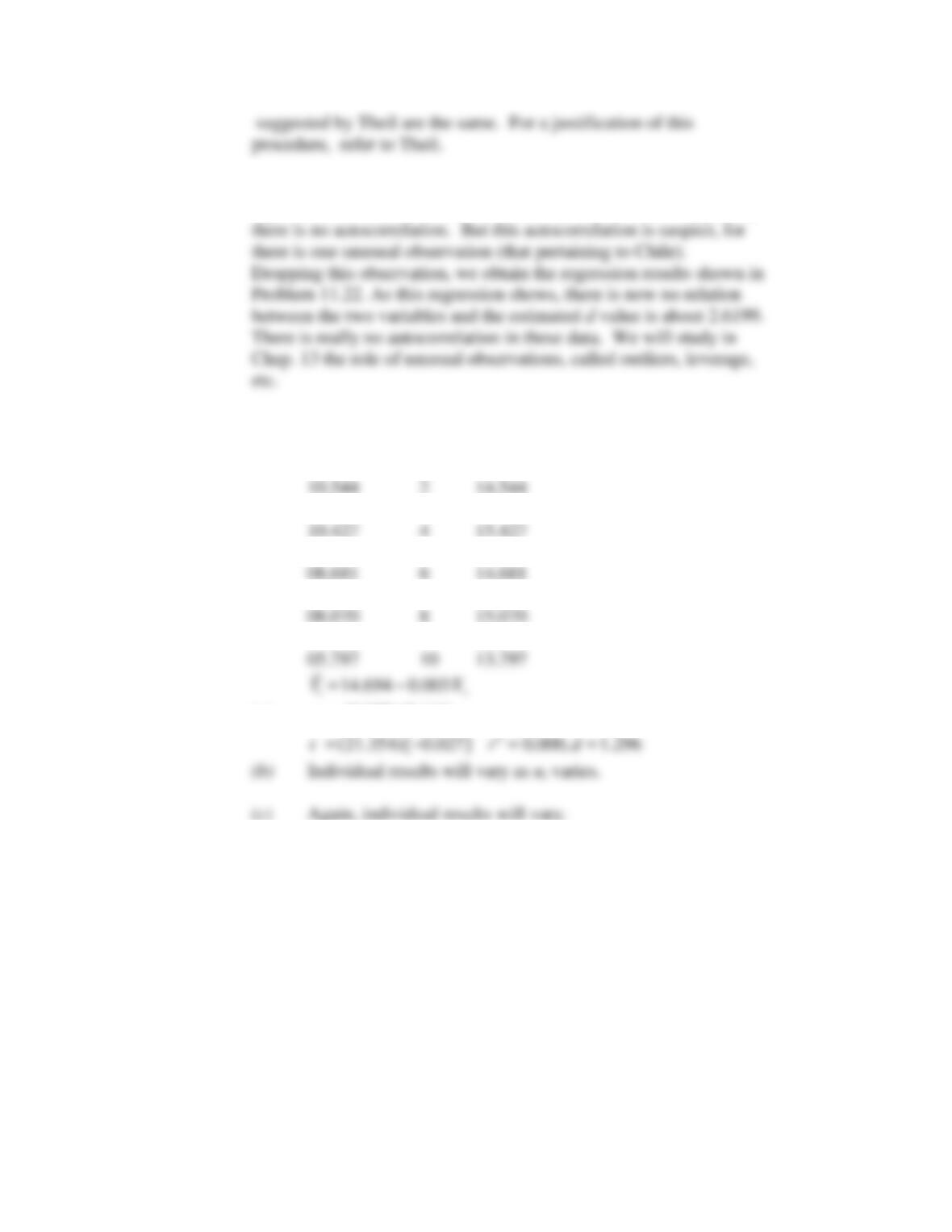
12.33
One set of data generated by the suggested scheme is as follows:
u
t
X
t
Y
t
09.464 1 12.964
11.944 3 16.444
09.316 5 14.816
07.525 7 14.025
07.504 9 15.004
(a)
(0.688) (0.111)
se
=
12.34
(a) The results of the regression of inventory on sales, each in
millions of dollars, are:
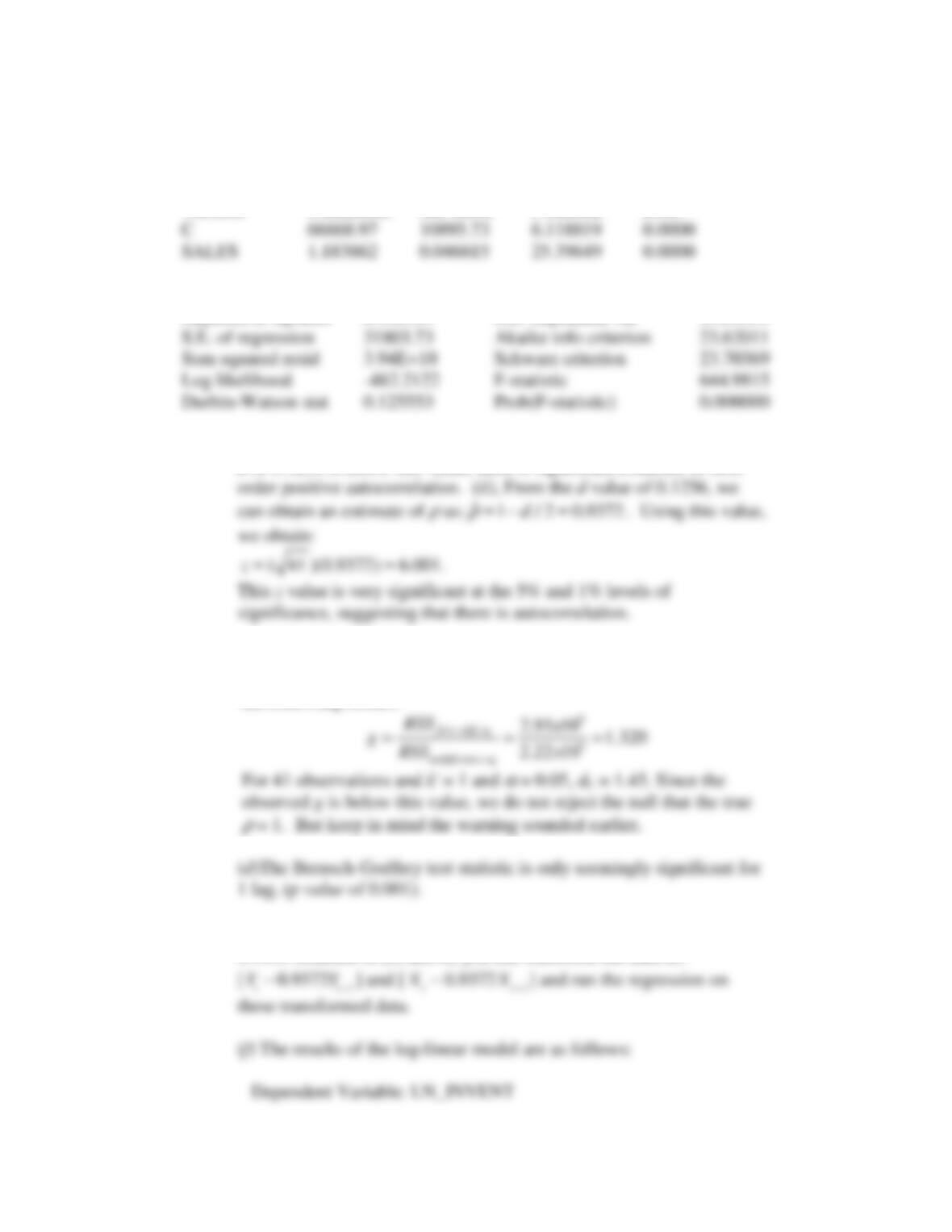
Basic Econometrics, Gujarati and Porter
154
Dependent Variable: INVENTORIES
Sample: 1950 1990
Included observations: 41
Variable Coefficient Std. Error t-Statistic Prob.
R-squared 0.942981 Mean dependent var 312958.1
Adjusted R-squared 0.941519 S.D. dependent var 131513.5
(b) (i) For n = 42, k‘ = 1, the 5% d
L
is 1.46. Since the observed
d of 0.1256 is below this value, there is significant evidence of first-
(c) In view of the results in (b) it does seem possible that the
the true
ρ
is one. But if you mechanically apply the test, we get
the following results:
(e)If you use only the first-order AR scheme, using the
ρ
value of
0.9416 obtained in (b) above, you can transform the data as:
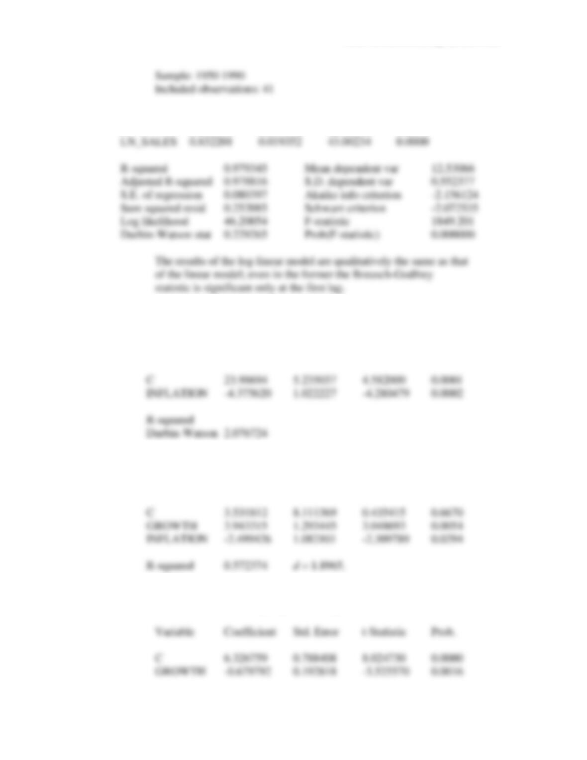
Basic Econometrics, Gujarati and Porter
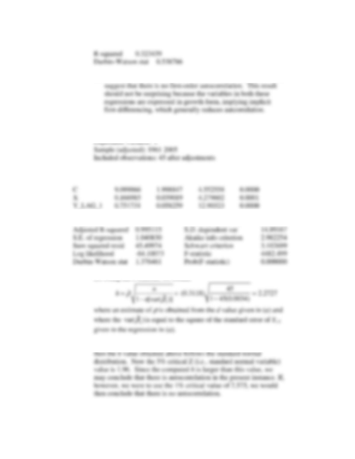
155
Variable Coefficient Std. Error t-Statistic Prob.
C 2.486980 0.233898 10.63274 0.0000
(g) See the discussion in Chap. 6 and Sec. 8.11.
12.35
(a) The regression results are as follows:
Variable Coefficient Std. Error t-Statistic Prob.
(b)
Variable Coefficient Std. Error t-Statistic Prob.
(d)
Fama’s statement is correct. To see this further, regressing
current inflation on output growth, we get:
Basic Econometrics, Gujarati and Porter
156
(e)
In both these regressions the d values are around 2, which would
12.36
(a) The regression results are:
Variable Coefficient Std. Error t-Statistic Prob.
R-squared 0.995337 Mean dependent var 91.11111
(b) Using the h statistic, we obtain:
If we assume the sample size of 45 observations as reasonably large,
157
12.37
The regression results based on the Maddala procedure discussed
in the text are as follows:
Variable Coefficient Std. Error t-Statistic Prob.
C -4.041785 23.34284 -0.173149 0.8642
R-squared 0.551249
12.38
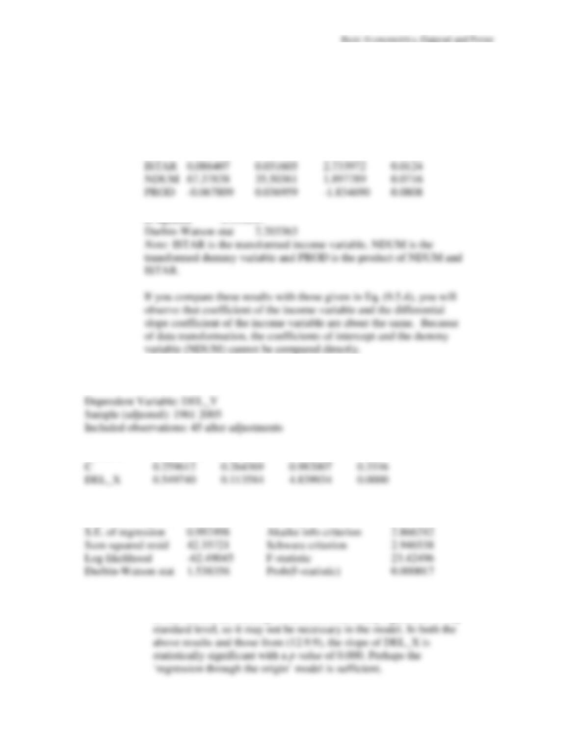
Regression results for the model in (12.9.8) are as follows:
Variable Coefficient Std. Error t-Statistic Prob.
R-squared 0.352653 Mean dependent var 1.320000
Adjusted R-squared 0.337598 S.D. dependent var 1.219463
Where DEL_Y is
VY
t
=Y
t
−Y
t−1
and DEL_X is
VX
t
=X
t
−X
t−1
.
In this model, the intercept term is not statistically significant at any